IBM AC922 서버에서 CUDA-enabled HPL 수행하기

HPL (High Performance Linpack) 테스트는 수퍼컴 클러스터의 성능 측정에 널리 쓰이는 오픈소스 프로그램입니다.   GPU를 사용하여 HPL을 수행하기 위해서는 CUDA-enabled HPL이 필요한데, 그건 NVIDIA가 지적 재산권을 가진 프로그램이며 그건 오픈소스가 아닙니다.  WWW 상을 뒤져보면 CUDA-enabled HPL의 source code를 NVIDIA가 공개하기는 하는데, 그건 매우 오래된 GPU architecture인 Fermi 아키텍처의 GPU에 대한 것이라서 최신 GPU의 성능 측정에는 적절하지 않습니다.

아래에서는 NVIDIA의 협조를 받아 CUDA-enabled HPL의 executible binary file을 가지고 있다는 전제 하에 IBM AC922 서버 (POWER9 * 2, V100 SXM2 32GB GPU * 4) 1대로 CUDA-enabled HPL을 수행하는 과정만 제시합니다.

그 결과는 역시 confidential 정보라 공개하지 못하는 점 양해 부탁드립니다.

이 테스트 수행을 위해서는 서버에 먼저 CUDA 10.1이 설치되어 있어야 합니다.  또한 IBM의 XL Fortran, Spectrum MPI, ESSL 등의 library 등이 필요합니다.

[cecuser@p1235-met1 HPC]$ ls
ESSL_FOR_LINUX_ON_POWER_V6.2.0.tar.gz
hpl_cuda10.1.4gpus.tgz
IBM_SMPI_10.2_IP_GR_LINUX_PPC64LE.tgz
ibm_smpi_lic_s-10.02-p9-ppc64le.rpm
lsf10.1_lnx310-lib217-ppc64le.tar.Z
XL_FORTRAN_FOR_LINUX_V16.1.1_PRO.gz

먼저 XL Fortran을 설치합니다.

[cecuser@p1235-met1 HPC]$ mkdir xlf

[cecuser@p1235-met1 HPC]$ cd xlf

[cecuser@p1235-met1 xlf]$ tar -zxvf ../XL_FORTRAN_FOR_LINUX_V16.1.1_PRO.gz

[cecuser@p1235-met1 xlf]$ ./install
...
Press Enter to continue viewing the license agreement, or, Enter "1" to accept the agreement,
"2" to decline it or "99" to go back to the previous screen, "3" Print.
1
INFORMATIONAL: Unexpected CUDA Toolkit version detected '10.1' (9.2, 10.0 are supported), defaulting to __CUDA_API_VERSION=10000.  Re-configure with '-cudaVersion 9.2' to override.
Installation and configuration successful


이어서 Spectrum MPI를 설치합니다.  10.1이 아니라 10.2가 필요합니다.

[cecuser@p1235-met1 HPC]$ tar -zxf IBM_SMPI_10.2_IP_GR_LINUX_PPC64LE.tgz

[cecuser@p1235-met1 HPC]$ cd ibm_smpi-10.02.00.03-p9-ppc64le

[cecuser@p1235-met1 ibm_smpi-10.02.00.03-p9-ppc64le]$ sudo rpm -Uvh *.rpm ../ibm_smpi_lic_s-10.02-p9-ppc64le.rpm

[cecuser@p1235-met1 ibm_smpi-10.02.00.03-p9-ppc64le]$ su -

[root@p1235-met1 ~]# IBM_SPECTRUM_MPI_LICENSE_ACCEPT=yes /opt/ibm/spectrum_mpi/lap_se/bin/accept_spectrum_mpi_license.sh

[root@p1235-met1 ~]# exit

이어서 ESSL을 설치합니다.  이건 engineering용 library인데, GPU를 이용하도록 되어 있습니다.

[cecuser@p1235-met1 HPC]$ tar -zxvf ESSL_FOR_LINUX_ON_POWER_V6.2.0.tar.gz

[cecuser@p1235-met1 HPC]$ cd RHEL/RHEL7/

[cecuser@p1235-met1 RHEL7]$ su
Password:

[root@p1235-met1 RHEL7]# rpm -Uvh essl.license-6.2.0-0.ppc64le.rpm

[root@p1235-met1 RHEL7]# export IBM_ESSL_LICENSE_ACCEPT=yes

[root@p1235-met1 RHEL7]# /opt/ibmmath/essl/6.2/lap/accept_essl_license.sh

[root@p1235-met1 RHEL7]# rpm -Uvh essl.3264.rte-6.2.0-0.ppc64le.rpm essl.6464.rte-6.2.0-0.ppc64le.rpm essl.rte.common-6.2.0-0.ppc64le.rpm essl.man-6.2.0-0.ppc64le.rpm essl.3264.rtecuda-6.2.0-0.ppc64le.rpm essl.common-6.2.0-0.ppc64le.rpm essl.msg-6.2.0-0.ppc64le.rpm essl.rte-6.2.0-0.ppc64le.rpm


이제 CUDA-enabled HPL의 binary 및 script를 풀어냅니다.

[cecuser@p1235-met1 HPC]$ tar -zxvf hpl_cuda10.1.4gpus.tgz

[cecuser@p1235-met1 HPC]$ cd hpl

이 속에 들어있는 것은 간단합니다.  Binary 실행 파일인 xhpl과 함께, 그 수행에 필요한 HPL.dat, 기타 mpirun을 위한 script 입니다.

먼저 HPL.dat의 내용입니다.  Edit해야 하는 주요 내용은 아래 붉은 색으로 표시한 Ns (계산해야 하는 문제의 크기), NBs (한번에 어느 정도 크기로 문제를 풀 것인지 결정하는 block size), 그리고 mesh 구조를 결정하는 Ps와 Qs입니다. 

간단히 말하면 Ns는 가급적 GPU들의 메모리를 꽤 가득 채울 정도로 크게 하고, NBs는 적절한 크기를 trial & error 방식으로 찾아야 합니다.  가령 제가 해보니 아래와 같은 크기의 Ns면 32GB memory의 GPU 4장을 가득 채웁니다.  또한 256이나 768에 비해 512로 NBs를 두는 것이 가장 성능이 잘 나오는 것 같습니다.  Ps와 Qs는 서로 곱해서 GPU 갯수가 나오면 되는데, 가급적 서로 비슷하게, 그리고 가급적 Ps가 Qs보다 작게 설정하면 됩니다.

[cecuser@p1235-met1 hpl]$ cat HPL.dat
HPLinpack benchmark input file
Innovative Computing Laboratory, University of Tennessee
HPL.out      output file name (if any)
6            device out (6=stdout,7=stderr,file)
1            # of problems sizes (N)
128000       Ns
1          # of NBs
512        NBs
0            PMAP process mapping (0=Row-,1=Column-major)
1            # of process grids (P x Q)
2            Ps
2            Qs
16.0         threshold
1            # of panel fact
2            PFACTs (0=left, 1=Crout, 2=Right)
1            # of recursive stopping criterium
4            NBMINs (>= 1)
1            # of panels in recursion
2            NDIVs
1            # of recursive panel fact.
0            RFACTs (0=left, 1=Crout, 2=Right)
1            # of broadcast
3            BCASTs (0=1rg,1=1rM,2=2rg,3=2rM,4=Lng,5=LnM)
1            # of lookahead depth
0            DEPTHs (>=0)
1            SWAP (0=bin-exch,1=long,2=mix)
192          swapping threshold
1            L1 in (0=transposed,1=no-transposed) form
0            U  in (0=transposed,1=no-transposed) form
0            Equilibration (0=no,1=yes)
8            memory alignment in double (> 0)

여기서는 1대로 수행하니까 hosts 파일은 사실 필요가 없습니다만 아래와 같은 format으로 설정하면 됩니다.

[cecuser@p1235-met1 hpl]$ cat hosts
localhost  slots=4

아래는 mpirun을 수행하는 script입니다.  제가 쓴 환경처럼 infiniband가 없는 경우 "-pami_noib" 옵션을 써야 합니다.

[cecuser@p1235-met1 hpl]$ cat run_me_4_gpu_xlc_spectrum.sh
#!/bin/bash
export MPI_ROOT=/opt/ibm/spectrum_mpi
export MANPATH=$MPI_ROOT/share/man:$MANPATH
export PATH=/usr/local/cuda-10.1/bin:/opt/ibm/spectrum_mpi/bin:$PATH
export LD_LIBRARY_PATH=/opt/ibmmath/essl/6.2/lib64/:/opt/ibm/spectrum_mpi/lib:$LD_LIBRARY_PATH
sudo nvidia-smi -ac 877,1395
#echo always > /sys/kernel/mm/transparent_hugepage/enabled
TUNE="-x PAMI_IBV_DEVICE_NAME=mlx5_0:1 -x PAMI_IBV_DEVICE_NAME_1=mlx5_3:1 -x PAMI_ENABLE_STRIPING=0 -x PAMI_IBV_CQEDEPTH=4096 -x PAMI_IBV_ADAPTER_AFFINITY=1 -x PAMI_IBV_OPT_LATENCY=1 -x MLX5_SINGLE_THREADED=1 -x MLX5_CQE_SIZE=128 -x PAMI_IBV_ENABLE_DCT=1 -x PAMI_IBV_ENABLE_OOO_AR=1 -x PAMI_IBV_QP_SERVICE_LEVEL=8"
sudo ppc64_cpu --dscr=7
#mpirun -N 4 -npernode 4 --allow-run-as-root -x OMPI_MCA_common_pami_use_odp=0 -x PAMI_IBV_DEBUG_PRINT_DEVICES=1 -tag-output $TUNE --hostfile nodes -bind-to none ./run_linpack_6_gpu_xlc_spectrum_0726
mpirun -N 4 -npernode 4 --hostfile hosts -pami_noib -bind-to none ./run_linpack_4_gpu_xlc_spectrum.sh


그리고 아래가 실제 xhpl을 수행하는 script입니다.  위의 mpirun script를 수행하면 결국 아래의 script가 수행됩니다.  IBM의 Spectrum MPI에서는 내부적으로 OMPI_COMM_WORLD_LOCAL_RANK, PMIX 등의 환경 변수를 자동 생성하여 GPU를 할당하는데 사용합니다.  아래 script를 보면 case 문을 이용하여 CUDA_VISIBLE_DEVICES 환경 변수를 이용하여 GPU 1개씩마다 xhpl을 하나씩 수행합니다.


[cecuser@p1235-met1 hpl]$ cat run_linpack_4_gpu_xlc_spectrum.sh
#!/bin/bash
#location of HPL
HPL_DIR=`pwd`
# Number of CPU cores
# Total CPU cores / Total GPUs (not counting hyperthreading)
#CPU_CORES_PER_RANK=16
CPU_CORES_PER_RANK=8
export MPI_ROOT=/opt/ibm/spectrum_mpi
export OMP_NUM_THREADS=$CPU_CORES_PER_RANK
export MAX_H2D_MS=10
export MAX_D2H_MS=10
export RANKS_PER_SOCKET=2
export RANKS_PER_NODE=4
export NUM_WORK_BUF=4
export SCHUNK_SIZE=128
export GRID_STRIPE=4
export FACT_GEMM=1
export FACT_GEMM_MIN=128
export SORT_RANKS=0
export PRINT_SCALE=1.0
export TEST_SYSTEM_PARAMS=1
sudo rm -rf /dev/shm/sh_*
export LIBC_FATAL_STDERR_=1
#export PAMI_ENABLE_STRIPING=0
export CUDA_CACHE_PATH=/tmp
export OMP_NUM_THREADS=$CPU_CORES_PER_RANK
export CUDA_DEVICE_MAX_CONNECTIONS=8
export CUDA_COPY_SPLIT_THRESHOLD_MB=1
export GPU_DGEMM_SPLIT=1.0
export TRSM_CUTOFF=1000000
#export TRSM_CUTOFF=99000
export TEST_SYSTEM_PARAMS=1
export MONITOR_GPU=1
export GPU_TEMP_WARNING=70
export GPU_CLOCK_WARNING=1310
export GPU_POWER_WARNING=350
export GPU_PCIE_GEN_WARNING=3
export GPU_PCIE_WIDTH_WARNING=2
#export ICHUNK_SIZE=1536
export ICHUNK_SIZE=384
export CHUNK_SIZE=5120
APP=$HPL_DIR/xhpl
#lrank=$OMPI_COMM_WORLD_LOCAL_RANK
lrank=$(($PMIX_RANK%4))
nrank=$(($PMIX_RANK/4))
#crank=$(($nrank/89))
#neven=$(($crank%2))
neven=$(($nrank%2))
#neven=0
export CUDA_VISIBLE_DEVICES=$lrank
echo "RANK $PMIX_RANK on host $HOSTNAME PID $$ even: $neven"
if [ $neven -eq 0 ]
then
case ${lrank} in
[0])
#ldd $APP
sudo nvidia-smi -ac 877,1395 > /dev/null;
#export PAMI_IBV_DEVICE_NAME=mlx5_0:1;
#export OMPI_MCA_btl_openib_if_include=mlx5_0:1;
export CUDA_VISIBLE_DEVICES=0; numactl --physcpubind=0,4,8,12,16,20,24,28,32,36 --membind=0 $APP
  ;;
[1])
#export PAMI_IBV_DEVICE_NAME=mlx5_1:1;
#export OMPI_MCA_btl_openib_if_include=mlx5_1:1;
export CUDA_VISIBLE_DEVICES=1; numactl --physcpubind=40,44,48,52,56,60,64,68,72,76 --membind=0 $APP
  ;;
[2])
#export PAMI_IBV_DEVICE_NAME=mlx5_0:1;
#export OMPI_MCA_btl_openib_if_include=mlx5_0:1;
export CUDA_VISIBLE_DEVICES=2; numactl --physcpubind=80,84,88,92,96,100,104,108,112,116 --membind=8 $APP
  ;;
[3])
#export PAMI_IBV_DEVICE_NAME=mlx5_3:1;
#export OMPI_MCA_btl_openib_if_include=mlx5_3:1;
export CUDA_VISIBLE_DEVICES=3; numactl --physcpubind=120,124,128,132,136,140,144,148,152,156 --membind=8 $APP
  ;;
esac
exit
fi


이제 다음과 같이 run_me_4_gpu_xlc_spectrum.sh를 수행하시면 됩니다.  대략 10분 이내의 시간이 걸릴 것입니다.

[cecuser@p1235-met1 hpl]$ ./run_me_4_gpu_xlc_spectrum.sh


중간값을 빼면 결과적으로는 아래와 같은 결과물이 display 됩니다.   결과는 공개하지 못하는 점 다시 한번 양해 부탁드립니다.

...

================================================================================
T/V                N    NB     P     Q               Time                 Gflops
--------------------------------------------------------------------------------
WR03L2R4      128000   512     2     2             XXX              X.XXXe+04
--------------------------------------------------------------------------------
||Ax-b||_oo/(eps*(||A||_oo*||x||_oo+||b||_oo)*N)=        0.0005540 ...... PASSED
================================================================================

H2O Driverless AI를 통한 인물별 의료비 예측

H2O Driverless AI (이하 H2O DAI)의 또다른 유력한 use case인 보험 업무에 대해 살펴보겠습니다.   보험사에게 있어 의료비가 많이 들 것 같은 사람을 골라내는 것은 보험사의 수익과 직결되는 무척 중요한 일입니다.  아래 Kaggle site에서 얻은 환자 기본 정보 및 각 환자에게 든 의료비에 대한 dataset을 이용하여 H2O DAI가 예상 의료비를 얼마나 정확히 측정하는지 테스트 해보겠습니다.

https://www.kaggle.com/mirichoi0218/insurance

이 dataset에는 다음과 같은 칼럼들이 있습니다. 

age  나이
sex  성별
bmi  비만도
children  자녀수
smoker  흡연여부
region  사는 지역
charges  의료비

보험사에서 예측하고 싶은 것은 물론 맨 마지막 칼럼인 charges 부분일 것입니다.  이제 H2O DAI를 이용하여 어떻게 이 dataset으로부터 특정 조건을 가진 인물의 예상 의료비를 뽑아낼 수 있는지 step by step으로 알아보시도록 하겠습니다.

1) 웹 브라우저를 통해 H2O DAI에 접속합니다.   맨 처음 menu는 'DATASET'이며, 여러가지 입력 방법 중에서 저는 제 laptop으로부터 upload하는 menu를 택하겠습니다.

2) 저는 위의 Kaggle dataset (insurance.csv)에서 미리 일부 row들을 떼어내어 insurance_test.xlsx를 만들었고, 그 나머지를 insurance_training.xlsx로 저장해놓았습니다.  이것들을 선택하여 H2O DAI에 dataset으로 등록합니다.

3) insurance_training.xlsx와 insurance_test.xlsx가 dataset으로 등록되었습니다.   우측의 'Click for Actions' 부분을 눌러 나오는 sub-menu 중 'DETAILS' 부분을 클릭해 봅니다.

4) 이 DETAILS' 메뉴에서는 이 dataset이 어떤 정보를 담고 있는지 보실 수 있습니다.  각 칼럼별 평균/최대/최소/편차 등의 기본 정보와 최초 20개 row의 값 등을 보실 수 있습니다. 

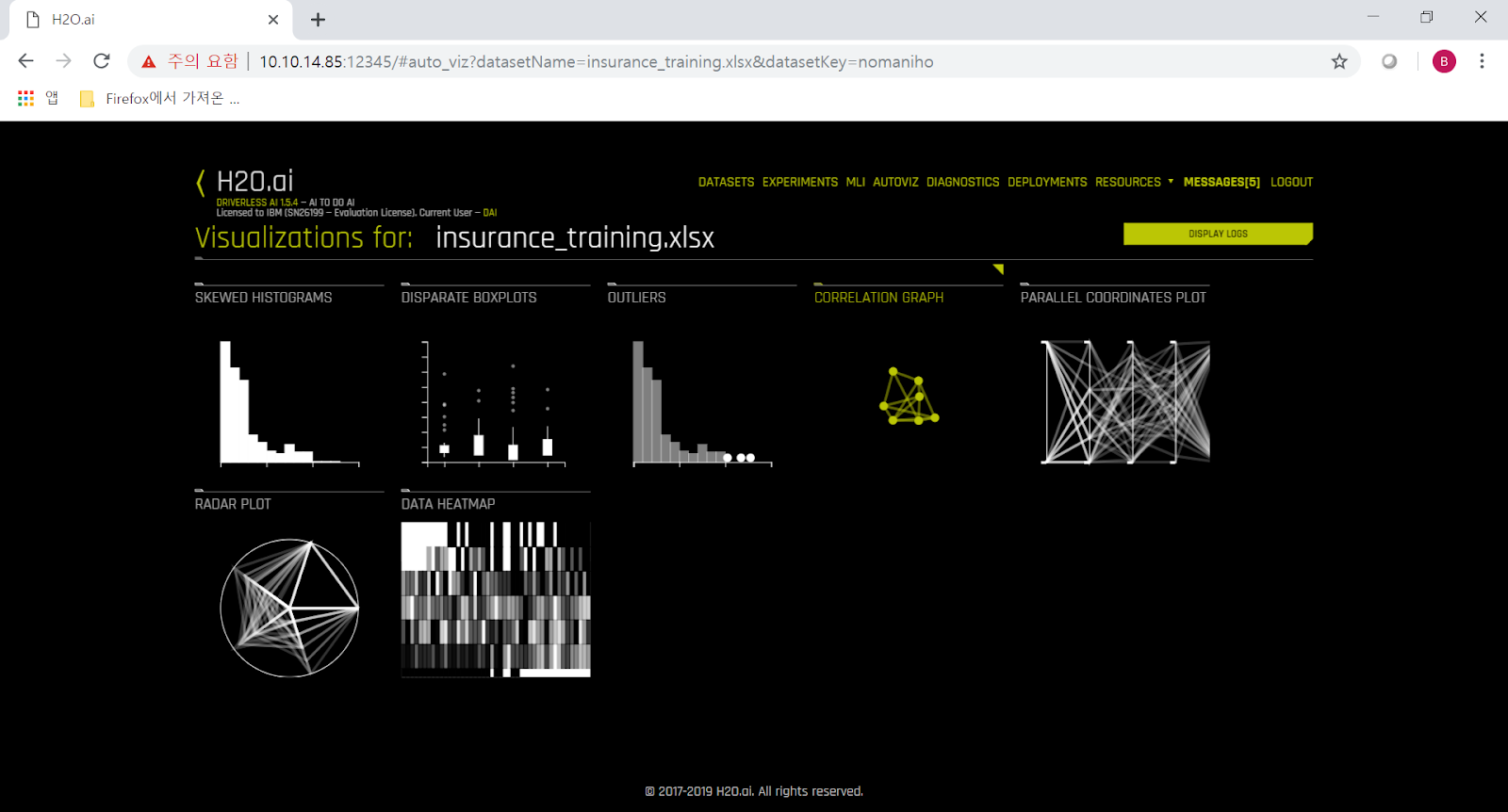
5) Dataset 우측의 'Click for Actions' 부분을 눌러 나오는 sub-menu 중 'VISUALIZATION'을 클릭하면 여러가지 다양한 graph가 자동으로 생성됩니다.   가령 'OUTLIERS PLOT'을 보면 전체 data 중 일부가 표준편차에서 크게 벗어난 것을 보실 수 있습니다.  그런 부분은 표에서 보는 것보다는 이렇게 그래프로 시각화해서 보면 직관적으로 이해하기가 쉽지요.  그렇게 크게 벗어난 오렌지색 점을 클릭해보면 해당 row의 상세 정보를 보실 수도 있습니다.

6) H2O DAI에서 가장 중요한 것은 역시 'PREDICT' 메뉴입니다.  이 메뉴를 통해서 예측 모델을 자동 생성하게 됩니다. 

7) 'PREDICT' 메뉴에 들어가면 꼭 하셔야 할 일은 단 하나 밖에 없습니다.  어느 칼럼에 대한 예측 모델을 만드느냐에 대한 선택입니다.  여기서는 당연히 charges 칼럼을 택합니다.

8) 추가로 선택하실 수 있는 메뉴는 중앙 하단의 3개의 라디오 다이얼입니다.  각각의 의미와 강약 조절은 아래와 같습니다.   여기서는 default로 제시된 8-3-8을 그대로 적용하겠습니다.

Accuracy : 어떤 알고리즘들을 몇 개나 적용할지 정합니다.  물론 다이얼 숫자가 높을 수록 더 많은 알고리즘을 적용합니다.
Time : 머신러닝에서 반복 훈련, 즉 iteration을 몇 회나 수행할지 정합니다.  물론 다이얼 숫자가 높을 수록 더 많은 회수가 적용됩니다.
Interpretability : 머신러닝으로 만들어진 모델에 대한 해석의 강도 조절 부분입니다.  다이얼 숫자가 높을 수록 더 단순화해서 해석해줍니다.


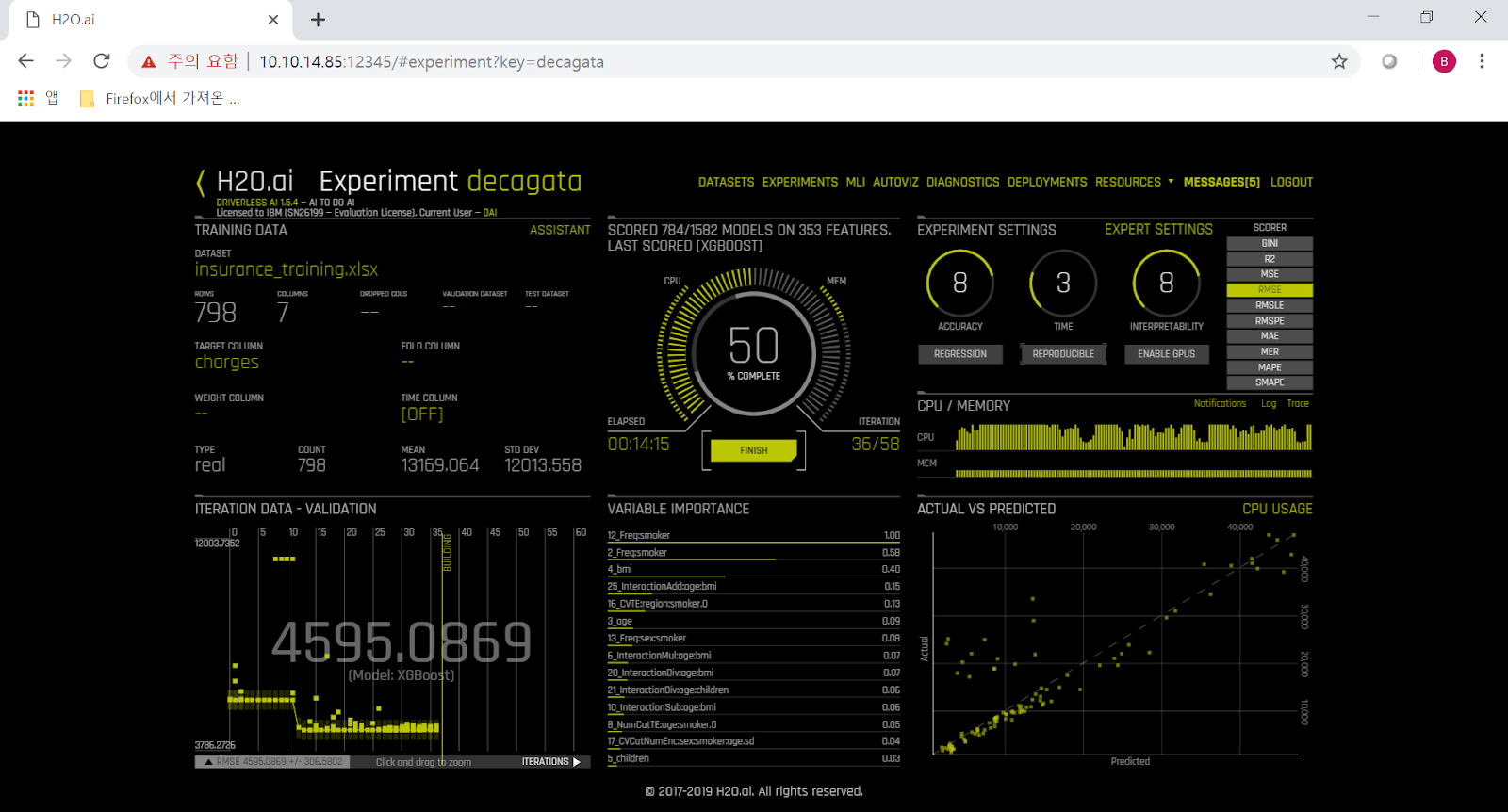
9) Launch를 누르면 자동 모델 생성이 시작되고 모델이 training 되는 과정을 보시게 됩니다.  중앙 상단을 보면 그 단계에서 하고 있는 작업과 적용되는 알고리즘 등이 실시간으로 업데이트 되면서 보여집니다.  중앙 하단에는 그 시점까지의 분석 단계에서 판단할 때 가장 중요한 변수/feature, 즉 입력된 dataset의 칼럼 중 어느 칼럼이 가장 중요한 역할을 하더라는 것이 실시간으로 분석되어 보여집니다.   가령 3% 경과된 시점에서는 LIGHTGBM 알고리즘을 처리 중이고, 흡연여부-비만지수-나이 순으로 병원비에 중요한 영향을 끼친다고 나옵니다. 

10) 그러나 auto feature engineering이 본격적으로 시작되면서 경과%가 진행되면서 그 값들은 계속 변화합니다.  가령 79% 경과 진행 중일 때는 무려 497개의 feature에 대해 1582개의 model에 대해서 평가 중이라고 나오지요.  원래 dataset의 칼럼 수, 즉 feature 수가 7개 밖에 없었다는 점을 생각하면 H2O DAI가 정말 다양한 조합의 feature engineering을 자동으로 수행하고 있다는 점을 아실 수 있습니다.  그 결과로 나오는 중앙 하단의 'Variable Importance', 즉 어떤 변수/feature가 병원비 지출액에 가장 중요한 영향을 끼치더라는 점도 비만도와 성별, 그리고 흡연여부가 결합되어 새로 생성된 변수를 가장 중요시하는 것을 보실 수 있습니다.  그 항목들을 자세히 보시면, 정말 모든 경우에 흡연여부가 가장 중요한 영향을 끼친다는 것을 보실 수 있습니다.  흡연인 여러분, 아무래도 담배는 끊으셔야 할 것 같습니다.

11) 모델 생성이 완료되면 우측 하단에 요약 설명이 나옵니다.  그러나 가장 중요한 것은 중앙 상단 메뉴의 3번쨰 항목, 즉 'SCORE ON ANOTHER DATASET' 입니다.  여기에 우리가 원하는 charges 값을 뺀 다른 값들 (연령, 사는 곳, 성별, 흡연 여부 등)이 들어있는 표를 입력하면, 해당 사람들이 얼마나 병원비를 쓸지 예측한 값을 출력해주거든요.   여기서는 미리 입력해둔 insurance_test.xlsx를 test dataset으로 선택하겠습니다.  그러면 곧장 해당 사람들의 병원비(charges) 값을 예측하여 그 결과를 csv 파일로 download 시켜줍니다.

12) 그렇게 해서 얻은 해당 환자들의 예상 병원비와 실제 병원비의 결과는 아래 그래프와 같습니다.  파란 곡선이 실제값이고, 오렌지색 곡선이 H2O DAI가 예측한 값입니다.  놀랍도록 잘 맞춘 것을 보실 수 있습니다.   다만 중간 정도에 H2O DAI는 7천4백불 정도를 예상했는데 실제로는 2만8천불을 사용하여 H2O DAI의 예상이 크게 틀린 환자가 있습니다.  이 환자의 상태를 보면, BMI 지수가 높은 비흡연자입니다.  아마도 H2O DAI가 만든 모델에서는 BMI 지수는 그다지 중요하지 않고 흡연 여부가 가장 중요했는데, 이 환자의 경우는 그 예측이 빗나간 것 같습니다.

13) 위에서 BMI 지수니 흡연여부니 하는 것은 어디까지나 저 개인의 짐작에 불과할 뿐 수학적인 모델로 계산한 결과는 아닙니다.  왜 이 머신러닝 모델이 이런 예측값을 내놓았는지 해석하는 것이 바로 MLI (Machine Learning Interpretation)입니다.  H2O는 K-LIME과 Decision Tree, Random Forest 등 다양한 MLI 기능을 제공합니다.  그런 MLI는 모델 생성 완료시의 메뉴 맨 상단의 'Interpret This Model'을 클릭함으로써 생성할 수 있습니다. 

14) 이런 MLI 해석 결과도 어느 정도 data science에 대한 소양이 있어야 볼 수 있는 것이 사실입니다.  가령 LIME이 무엇인지 알아야 이해를 할 수 있으니까요.  (참고로 LIME은 Locally Interpretable Model-agnostic Explainations을 뜻하는 말로서, 어떤 모델을 생성할 때 사용된 변수 값을 하나씩 바꿔보고 그 모델의 결과에 얼마나 변화가 생기는지 봄으로써 어느 변수가 가장 중요한 역할을 하는지 해석하는 기법입니다.)  하지만 H2O DAI는 일반인들도 이해하기 쉬운 설명도 제시합니다.

15) 가령 Summary 부분의 맨 아래는 원래 dataset의 칼럼 중에서 어느 칼럼이 가장 중요한 역할을 하는지 보여줍니다. 

16) KLIME에서는 각각의 예측값에 대해, 어떤 변수가 어느 정도의 영향을 끼쳤는지를 수식화해서 보여줍니다.

17) 가장 쉬운 설명은 KLIME 메뉴 중 중앙상단의 'Explanations' 버튼을 클릭하면 볼 수 있습니다.   여기서는 흡연여부, BMI 지수 등의 변수의 증감에 따라 우리가 알고자 하는 target (여기서는 병원비)의 증감이 어떻게 변화하는지 최대한 단순화하여 제시합니다.  여기에 제시된 설명에 따르면 흡연여부가 가장 중요하고, 자녀가 있는지 여부가 그 다음이며, 사는 곳이 어디인지도 꽤 큰 영향을 미치는 것 같습니다.  아마 부유한 동네인지 또는 그 지방의 식습관 등이 영향을 주는 것일까요 ?  왜 그런지 모르겠습니다만 이 예측 모델에서는 의외로 BMI 지수, 즉 비만 여부는 상대적으로 그다지 큰 영향을 주지는 않는다고 판단하고 있습니다.

이 포스팅의 결론은 다음과 같습니다.

1. H2O DAI는 무척 정확한 예측 모델을 정말 쉽게 만들어낼 수 있을 뿐만 아니라, 왜 그런 예측을 했는지도 매우 쉽게 풀어서 설명해줍니다.  
2. 흡연자 여러분, 금연 합시다.

ppc64le 환경에서 tensorflow 1.12를 source로부터 build 하기

Tensorflow v1.12는 IBM PowerAI toolkit v1.5.4에 포함되어 있습니다.  그러나 그건 CUDA 10.0 환경을 위해 만들어진 것이라서, CUDA 9.2 환경을 그대로 쓰고자 하는 고객분들께서는 사용하실 수 없습니다.  하지만 github의 source code로부터 직접 build하시면 간단합니다.

제가 build한 환경은 Anaconda3 5.2 (python 3.6.8) + CUDA 9.2 + NCCL 2.2 + CUDNN 7.4.1 + Redhat 7.4 ppc64le 입니다. 

먼저 아래와 같이 기초적으로 필요한 OS package들을 yum으로 설치하십시요.

[bsyu@redhat74 files]$ which python
~/anaconda3/bin/python

[bsyu@redhat74 files]$ python
Python 3.6.5 |Anaconda, Inc.| (default, Apr 29 2018, 16:38:54)
[GCC 7.2.0] on linux

[bsyu@redhat74 files]$ sudo yum install java-1.8.0-openjdk-devel.ppc64le zip unzip automake autoconf make gcc patch

[bsyu@redhat74 files]$ conda install protobuf wheel numpy six

Tensorflow v1.12 build를 위해서는 bazel v0.15 이상이 필요합니다.  Bazel v0.15를 bootstrap 방식으로 먼저 build합니다.  예전에는 ppc64le 환경에서 bazel을 build하는 것이 매우 힘들었는데, 이젠 x86_64 환경에서와 똑같이 그냥 build하시면 됩니다.

[bsyu@redhat74 files]$ wget https://github.com/bazelbuild/bazel/releases/download/0.15.0/bazel-0.15.0-dist.zip

[bsyu@redhat74 files]$ mkdir bazel-0.15 && cd bazel-0.15

[bsyu@redhat74 bazel-0.15]$ unzip ../bazel-0.15.0-dist.zip

[bsyu@redhat74 bazel-0.15]$ export EXTRA_BAZEL_ARGS="--host_javabase=@local_jdk//:jdk"

[bsyu@redhat74 bazel-0.15]$ export PROTOC=~/anaconda3/bin/protoc

[bsyu@redhat74 bazel-0.15]$ ./compile.sh
....
INFO: Build completed successfully, 2371 total actions
WARNING: --batch mode is deprecated. Please instead explicitly shut down your Bazel server using the command "bazel shutdown".
Build successful! Binary is here: /home/bsyu/files/bazel-0.15/output/bazel

이제 bazel build가 완료되었습니다.  이렇게 만든 bazel 실행파일을 아래와 같이 /usr/local/bin에 옮겨놓고 쓰시면 됩니다.

[bsyu@redhat74 bazel-0.15]$ sudo cp output/bazel /usr/local/bin

그리고 tensorflow build에 들어가기 전에, 아래와 같이 cudnn.h의 soft link를 /usr/include 밑에 만들어 줍니다.  이것이 없으면 자꾸 cudnn.h를 못 찾는다는 error("Cannot find cudnn.h under /usr/local/cuda-9.2/targets/ppc64le-linux/lib")가 나니까, 그걸 막기 위한 것입니다. 

[bsyu@redhat74 files]$ sudo ln -s /usr/local/cuda/include/cudnn.h /usr/include/cudnn.h

이제 tensorflow source code를 받습니다.

[bsyu@redhat74 files]$ git clone https://github.com/tensorflow/tensorflow.git

[bsyu@redhat74 files]$ cd tensorflow/

우리가 원하는 버전인 v1.12.0으로 checkout 합니다.

[bsyu@redhat74 tensorflow]$ git checkout tags/v1.12.0

./configure를 수행하되, 다음 몇 줄 이외에는 모두 default 값을 쓰면 됩니다.

[bsyu@redhat74 tensorflow]$ ./configure

Do you wish to build TensorFlow with CUDA support? [y/N]: y
Please specify the CUDA SDK version you want to use. [Leave empty to default to CUDA 9.0]: 9.2
Please specify the location where cuDNN 7 library is installed. Refer to README.md for more details. [Default is /usr/local/cuda]: /usr/local/cuda/lib64
Please note that each additional compute capability significantly increases your build time and binary size. [Default is: 3.5,7.0]: 6.0,7.0

그리고 temp file을 쓸 directory를 별도로 지정해두기 위해 다음과 같이 환경변수 TMP를 넉넉한 disk 공간이 있는 directory로 지정해두는 것이 좋습니다.

[bsyu@redhat74 tensorflow]$ export TMP=/data/tmp

이제 bazel을 이용하여 tensorflow build에 들어갑니다.  이 과정은 시간이 오래 걸리니까 nohup & 을 쓰시는 것이 좋습니다.   그리고 의외로 system memory를 많이 잡아먹습니다.  저는 16GB memory가 있는 POWER8 가상머신에서 했는데, active memory를 거의 9GB 쓰는 것 같습니다.   4GB memory만 있는 가상머신에서 build하려니 killed 되던데, 아마 메모리 부족으로 죽는 것 같았어요.

[bsyu@redhat74 tensorflow]$ bazel build --config=opt --config=cuda //tensorflow/tools/pip_package:build_pip_package
...
INFO: Build completed successfully, 1180 total actions

성공적으로 완료되었습니다.  이제 wheel file을 생성합니다.

[bsyu@redhat74 tensorflow]$ ./bazel-bin/tensorflow/tools/pip_package/build_pip_package /tmp/tensorflow_pkg
...
Fri Feb 22 22:05:17 KST 2019 : === Output wheel file is in: /tmp/tensorflow_pkg

이제 wheel file이 /tmp/tensorflow_pkg 밑에 생성되었습니다.   다음과 같이 확인합니다.

[bsyu@redhat74 tensorflow]$ ls -l /tmp/tensorflow_pkg
-rw-rw-r-- 1 bsyu bsyu 171252634 Feb 22 22:05 tensorflow-1.12.0-cp36-cp36m-linux_ppc64le.whl

이제 이 wheel file을 pip 명령으로 설치하면 됩니다.  이 과정 중에서 tensorflow에 필요한 grpcio 등의 python package들을 추가로 internet에서 download 하여 설치하므로, 만약 internet이 없는 환경이라면 intranet에 있는 PYPI repository에서 그런 package들을 download 할 수 있도록 설정이 필요합니다.

[bsyu@redhat74 tensorflow]$ pip install /tmp/tensorflow_pkg/tensorflow-1.12.0-cp36-cp36m-linux_ppc64le.whl

Processing /tmp/tensorflow_pkg/tensorflow-1.12.0-cp36-cp36m-linux_ppc64le.whl
Requirement already satisfied: numpy>=1.13.3 in /home/bsyu/anaconda3/lib/python3.6/site-packages (from tensorflow==1.12.0) (1.15.4)
Requirement already satisfied: keras-applications>=1.0.6 in /home/bsyu/anaconda3/lib/python3.6/site-packages (from tensorflow==1.12.0) (1.0.7)
Requirement already satisfied: keras-preprocessing>=1.0.5 in /home/bsyu/anaconda3/lib/python3.6/site-packages (from tensorflow==1.12.0) (1.0.9)
Requirement already satisfied: six>=1.10.0 in /home/bsyu/anaconda3/lib/python3.6/site-packages (from tensorflow==1.12.0) (1.12.0)
Requirement already satisfied: protobuf>=3.6.1 in /home/bsyu/anaconda3/lib/python3.6/site-packages (from tensorflow==1.12.0) (3.6.1)
Collecting termcolor>=1.1.0 (from tensorflow==1.12.0)
  Downloading https://files.pythonhosted.org/packages/8a/48/a76be51647d0eb9f10e2a4511bf3ffb8cc1e6b14e9e4fab46173aa79f981/termcolor-1.1.0.tar.gz
Collecting astor>=0.6.0 (from tensorflow==1.12.0)
  Downloading https://files.pythonhosted.org/packages/35/6b/11530768cac581a12952a2aad00e1526b89d242d0b9f59534ef6e6a1752f/astor-0.7.1-py2.py3-none-any.whl
Collecting grpcio>=1.8.6 (from tensorflow==1.12.0)
  Downloading https://files.pythonhosted.org/packages/90/2e/f432e69f86961393c22a6c4490aafdbb94533deba33f5ea2d5651770aa21/grpcio-1.18.0.tar.gz (14.6MB)
    100% |████████████████████████████████| 14.6MB 3.4MB/s
Collecting absl-py>=0.1.6 (from tensorflow==1.12.0)
  Downloading https://files.pythonhosted.org/packages/31/bc/ab68120d1d89ae23b694a55fe2aece2f91194313b71f9b05a80b32d3c24b/absl-py-0.7.0.tar.gz (96kB)
    100% |████████████████████████████████| 102kB 11.7MB/s
Collecting tensorboard<1.13.0,>=1.12.0 (from tensorflow==1.12.0)
  Downloading https://files.pythonhosted.org/packages/07/53/8d32ce9471c18f8d99028b7cef2e5b39ea8765bd7ef250ca05b490880971/tensorboard-1.12.2-py3-none-any.whl (3.0MB)
    100% |████████████████████████████████| 3.1MB 8.6MB/s
Collecting gast>=0.2.0 (from tensorflow==1.12.0)
  Downloading https://files.pythonhosted.org/packages/4e/35/11749bf99b2d4e3cceb4d55ca22590b0d7c2c62b9de38ac4a4a7f4687421/gast-0.2.2.tar.gz
Requirement already satisfied: wheel>=0.26 in /home/bsyu/anaconda3/lib/python3.6/site-packages (from tensorflow==1.12.0) (0.32.3)
Requirement already satisfied: h5py in /home/bsyu/anaconda3/lib/python3.6/site-packages (from keras-applications>=1.0.6->tensorflow==1.12.0) (2.7.1)
Requirement already satisfied: setuptools in /home/bsyu/anaconda3/lib/python3.6/site-packages (from protobuf>=3.6.1->tensorflow==1.12.0) (39.1.0)
Requirement already satisfied: werkzeug>=0.11.10 in /home/bsyu/anaconda3/lib/python3.6/site-packages (from tensorboard<1.13.0,>=1.12.0->tensorflow==1.12.0) (0.12.2)
Collecting markdown>=2.6.8 (from tensorboard<1.13.0,>=1.12.0->tensorflow==1.12.0)
  Downloading https://files.pythonhosted.org/packages/7a/6b/5600647404ba15545ec37d2f7f58844d690baf2f81f3a60b862e48f29287/Markdown-3.0.1-py2.py3-none-any.whl (89kB)
    100% |████████████████████████████████| 92kB 14.6MB/s
Building wheels for collected packages: termcolor, grpcio, absl-py, gast
  Running setup.py bdist_wheel for termcolor ... done
  Stored in directory: /home/bsyu/.cache/pip/wheels/7c/06/54/bc84598ba1daf8f970247f550b175aaaee85f68b4b0c5ab2c6
  Running setup.py bdist_wheel for grpcio ... done
  Stored in directory: /home/bsyu/.cache/pip/wheels/e5/22/5a/fa5c03beb66ecc2658e73673175e748ac37385614d52430877
  Running setup.py bdist_wheel for absl-py ... done
  Stored in directory: /home/bsyu/.cache/pip/wheels/90/db/f8/2c3101f72ef1ad434e4662853174126ce30201a3e163dcbeca
  Running setup.py bdist_wheel for gast ... done
  Stored in directory: /home/bsyu/.cache/pip/wheels/5c/2e/7e/a1d4d4fcebe6c381f378ce7743a3ced3699feb89bcfbdadadd
Successfully built termcolor grpcio absl-py gast
jupyter 1.0.0 requires qtconsole, which is not installed.
distributed 1.21.8 requires msgpack, which is not installed.
gevent 1.3.0 has requirement greenlet>=0.4.13, but you'll have greenlet 0.4.12 which is incompatible.
Installing collected packages: termcolor, astor, grpcio, absl-py, markdown, tensorboard, gast, tensorflow
Successfully installed absl-py-0.7.0 astor-0.7.1 gast-0.2.2 grpcio-1.18.0 markdown-3.0.1 tensorboard-1.12.2 tensorflow-1.12.0 termcolor-1.1.0

이제 보시는 바와 같이 tensorflow가 설치되었습니다.

[bsyu@redhat74 tensorflow]$ pip list | grep tensor
tensorboard                        1.12.2
tensorflow                         1.12.0

이걸 GPU가 있는 서버에서 테스트하는 방법은 다음과 같습니다.

[bsyu@redhat74 tensorflow]$ cd ..

[bsyu@redhat74 files]$ python
Python 3.6.8 |Anaconda, Inc.| (default, Dec 30 2018, 01:34:02)
[GCC 7.3.0] on linux

>>> import tensorflow as tf
/home/bsyu/anaconda3/lib/python3.6/site-packages/h5py/__init__.py:36: FutureWarning: Conversion of the second argument of issubdtype from `float` to `np.floating` is deprecated. In future, it will be treated as `np.float64 == np.dtype(float).type`.
  from ._conv import register_converters as _register_converters

>>> sess=tf.Session()
2019-02-22 22:14:15.250972: E tensorflow/stream_executor/cuda/cuda_driver.cc:300] failed call to cuInit: CUDA_ERROR_UNKNOWN: unknown error
2019-02-22 22:14:15.251021: I tensorflow/stream_executor/cuda/cuda_diagnostics.cc:150] kernel driver does not appear to be running on this host (redhat74): /proc/driver/nvidia/version does not exist

제가 GPU가 없는 서버에서 이걸 수행했기 때문에 위에서는 error가 났습니다만, GPU가 장착된 서버에서는 error가 없어야 하고 nvidia-smi로 보았을 때 python이 GPU를 점거하는 것으로 보일 것입니다.

여기서 build된 tensorflow wheel 파일과 site-packages directory 전체를 tar로 말아서 아래의 google drive에 올려두겠습니다.

tensorflow wheel 파일 : https://drive.google.com/open?id=1plqSuw9WnWuOPJCPEiVYSp3uK3IilQMy

CUDA 9.2의 AC922 서버에 tensorflow 1.12.0 설치하기

IBM POWER9 processor 기반의 GPU서버인 AC922을 2018년에 도입하셨던 고객분들은 대개 CUDA 9.2를 사용하고 계실 것입니다.  이 상황에서 아래와 같이 tensorflow를 포함한 기존 python package들의 버전을 올려야 하는 필요성이 있을 수 있습니다.

변경전 후
pandas 0.23.4  --> 0.24.0
tensorflow 1.8.0  --> 1.12.0
keras 2.2.2  --> 2.2.4
numpy 1.15.2  --> 1.16.1
scikit-learn 0.20.0  --> 0.20.2
scipy 1.0.0  --> 1.2.0

이게 가능할까요 ?  예 물론 가능합니다.  AC922 서버가 인터넷에 연결되어 있거나, 또는 사내 intranet에 PYPI (python repository) mirror본이 구성되어 있다면 쉽습니다.  (Tensorflow를 제외한 나머지 package들은) 아래와 같이 pip install --upgrade 명령을 통해 간단히 수행됩니다.

$ pip install --upgrade pandas==0.24.0
$ pip install --upgrade keras==2.2.4
$ pip install --upgrade numpy==1.16.1
$ pip install --upgrade scikit-learn==0.20.2
$ pip install --upgrade scipy==1.2.0

예를 들어 numpy는 아래와 같이 upgrade 됩니다.  설치 과정 때 nmon으로 시스템 모니터링을 해보면 cc1 (compiler)가 CPU를 열심히 쓰고 있는 것을 보실 수 있습니다.

[u0017649@sys-97058 files]$ pip install --upgrade numpy==1.16.1
Collecting numpy==1.16.1
  Downloading https://files.pythonhosted.org/packages/2b/26/07472b0de91851b6656cbc86e2f0d5d3a3128e7580f23295ef58b6862d6c/numpy-1.16.1.zip (5.1MB)
    100% |????????????????????????????????| 5.1MB 3.7MB/s
Building wheels for collected packages: numpy
  Running setup.py bdist_wheel for numpy ... done
  Stored in directory: /home/u0017649/.cache/pip/wheels/04/64/e1/283a3672c2865608968594c02a6923311f44d033bcece2683b
Successfully built numpy
jupyter 1.0.0 requires qtconsole, which is not installed.
distributed 1.21.8 requires msgpack, which is not installed.
gevent 1.3.0 has requirement greenlet>=0.4.13, but you'll have greenlet 0.4.12 which is incompatible.
Installing collected packages: numpy
  Found existing installation: numpy 1.13.3
    Uninstalling numpy-1.13.3:
      Successfully uninstalled numpy-1.13.3
Successfully installed numpy-1.16.1
You are using pip version 10.0.1, however version 19.0.2 is available.
You should consider upgrading via the 'pip install --upgrade pip' command.


문제는 tensorflow입니다.  Tensorflow는 불행히도 아직 1.12 버전이 ppc64le 아키텍처 상에서는 PYPI로부터는 pip로 설치가 안 됩니다.  하지만 이것도 큰 문제는 아닙니다.  Tensorflow는 open source니까, 그냥 github에서 source code를 받아서 직접 build하시면 됩니다.

원래 IBM은 작년 11월에 나온 PowerAI toolkit v1.5.4에서 tensorflow 1.12를 지원합니다.  그러나 이 PowerAI v1.5.4는 CUDA 10.0을 필요로 합니다.  따라서 이 PowerAI v1.5.4에 포함된 tensorflow를 쓰시려면 기존의 CUDA 9.2 환경을 뒤집어 엎고 CUDA 10.0으로 upgrade를 하셔야 합니다.  이건 기존에 쓰시던 다른 python package들과도 연관되는 일이니 그렇게 간단히 진행하실 일은 아니지요.

그래서 제가 tensorflow v1.12를 Redhat 7.4 ppc64le 플랫폼에서 python 3.6.8 + CUDA 9.2 환경용으로 build했고, 그 wheel file을 아래 google drive에 올려놓았습니다.  제가 가난하여 GPU 서버가 없는지라 test된 것은 아니라는 점은 양해 부탁드립니다. 

tensorflow v1.12 wheel file  --> https://drive.google.com/open?id=1plqSuw9WnWuOPJCPEiVYSp3uK3IilQMy

위의 wheel file을 download 받아서 아래 명령으로 설치하시면 됩니다.

[u0017649@sys-97058 files]$ pip install /tmp/tensorflow-1.12.0-cp36-cp36m-linux_ppc64le.whl

단 위의 tensorflow-*.whl 파일을 설치하실 때 pip가 termcolor, astor, grpcio 등의 필요 python package들을 추가로 internet에서 download하여 설치하므로, 만약 internet이 없는 환경이라면 intranet에 있는 PYPI repository에서 그런 package들을 download 할 수 있도록 설정이 필요하다는 점 유의하십시요.

설치가 끝난 뒤 확인하는 방법은 다음과 같습니다.

[bsyu@redhat74 tensorflow]$ pip list | grep tensor
tensorboard                        1.12.2
tensorflow                         1.12.0

[bsyu@redhat74 files]$ python
Python 3.6.8 |Anaconda, Inc.| (default, Dec 30 2018, 01:34:02)
[GCC 7.3.0] on linux

>>> import tensorflow as tf
/home/bsyu/anaconda3/lib/python3.6/site-packages/h5py/__init__.py:36: FutureWarning: Conversion of the second argument of issubdtype from `float` to `np.floating` is deprecated. In future, it will be treated as `np.float64 == np.dtype(float).type`.
  from ._conv import register_converters as _register_converters

>>> sess=tf.Session()
2019-02-22 22:14:15.250972: E tensorflow/stream_executor/cuda/cuda_driver.cc:300] failed call to cuInit: CUDA_ERROR_UNKNOWN: unknown error
2019-02-22 22:14:15.251021: I tensorflow/stream_executor/cuda/cuda_diagnostics.cc:150] kernel driver does not appear to be running on this host (redhat74): /proc/driver/nvidia/version does not exist

제가 GPU가 없는 서버에서 이걸 수행했기 때문에 위에서는 error가 났습니다만, GPU가 장착된 서버에서는 error가 없어야 하고 nvidia-smi로 보았을 때 python이 GPU를 점거하는 것으로 보일 것입니다.


PS1.  혹시 위의 wheel file 설치가 무슨 이유로든 잘 안 될 경우에 대비하여, 최후의 수단으로 tensorflow 및 위에 언급된 버전의 전체 python package들을 포함한 anaconda3 directory 전체를 tar로 말아서 아래의 google drive에 올려두겠습니다.

anaconda3 directory 전체의 tarball : https://drive.google.com/open?id=1vnmi8t2L_XKgRqfhQbBQbJgjVU7vNGav

위의 anaconda3_tf1.12.tgz를 다음과 같이 기존 anaconda3 directory 위치 또는 $HOME 밑에서 풀어놓으면 됩니다.  기존의 anaconda3 directory는 mv 명령으로 잠시 다른 이름으로 바꿔 놓으셨다가, 혹시 이 새로운 anaconda3가 정상 작동하지 않을 경우 다시 원복시키시기를 권고드립니다.

[root@sys-97264 opt]# ls
anaconda3   at11.0  ibm

[root@sys-97264 opt]# tar -zcpsf opt_anaconda3_tf1.12.tgz ./anaconda3

이 opt_anaconda3_tf1.12.tgz를 다른 서버에 올려놓은 뒤에 풀어놓아 보았습니다.  먼저 기존 anaconda3를 다른 이름으로 바꿔놓습니다.

[root@sys-97269 ~]# cd /opt

[root@sys-97269 ~]# mv anaconda3 anaconda3_org

[root@sys-97269 opt]# tar -zxvpsf /tmp/opt_anaconda3_tf1.12.tgz

[root@sys-97269 opt]# which python
/opt/anaconda3/bin/python

아래와 같이 잘 작동하는 것을 보실 수 있습니다.

[root@sys-97269 opt]# pip list | egrep 'pandas|Keras|numpy|scikit-learn|scipy|tensorflow'

Keras                              2.2.4

Keras-Applications                 1.0.7

Keras-Preprocessing                1.0.9

numpy                              1.16.1

numpydoc                           0.8.0

pandas                             0.24.0

scikit-learn                       0.20.2

scipy                              1.2.0

tensorflow                         1.12.0

[root@sys-97269 opt]# cd
[root@sys-97269 ~]# which python
/opt/anaconda3/bin/python

[root@sys-97269 ~]# python
Python 3.6.5 |Anaconda, Inc.| (default, Apr 29 2018, 16:38:54)
[GCC 7.2.0] on linux

>>> import keras
/opt/anaconda3/lib/python3.6/site-packages/h5py/__init__.py:36: FutureWarning: Conversion of the second argument of issubdtype from `float` to `np.floating` is deprecated. In future, it will be treated as `np.float64 == np.dtype(float).type`.
  from ._conv import register_converters as _register_converters
Using TensorFlow backend.
>>> import numpy
>>> import pandas
>>> import tensorflow
>>>

PS2.  혹시 위의 anaconda3 directory를 통째로 풀어놓는 것이 무슨 이유에서든 잘 안될 경우에 대비해서, 아래 site에 해당 tensorflow 등의 pacakge들을 모두 갖춘 CUDA 9.2를 설치한 Redhat 7.5 ppc64le 기반의 docker image를 올려놓았습니다.

https://hub.docker.com/r/bsyu/rhel75_ppc64le_cuda92_tf1.12_py3

다음과 같이 받아서 사용하시면 됩니다.

[u0017649@sys-97269 ~]$ sudo docker pull bsyu/rhel75_ppc64le_cuda92_tf1.12_py3:v0.2

ppc64le Redhat 서버에서 x86 hadoop cluster에 대해 hive로 query 수행하기

POWER9 CPU와 V100 GPU를 장착한 AC922 서버를 deep learning 용도로 사용하는 환경에서, training에 필요한 dataset은 x86 Cloudera hadoop cluster로부터 가져와야 할 필요가 있을 수 있습니다.

그런 경우, 방법은 크게 2가지가 있습니다.  하나는 그냥 hadoop 본연의 기능을 이용하는 것이고, 나머지 하나는 PyHive를 이용하는 것입니다.  이 포스팅에서는 hadoop 본연의 기능을 이용하는 방법을 먼저 다루겠습니다.  Pyhive를 이용하는 방법은 다음 posting에서 정리하겠습니다.

Hadoop 본연의 기능을 이용하려면 (당연히) ppc64le에 hadoop과 hive를 설치해야 합니다.  여기서는 접근해야 하는 x86 hadoop cluster에 Cloudera 5.14가 설치되어 있다고 가정하겠습니다.  CDH 5.14에는 hadoop 2.6.0과 hive 1.10이 들어있습니다.

먼저, ppc64le용 hadoop과 hive를 source로부터 build 합니다.  이 포스팅에 올려놓은 것처럼 source에서 직접 build하셔도 되고, 제가 미리 build해놓은 것을 download 받아 적절한 directory에 풀어놓기만 해도 됩니다.  제가 build 해놓은 것은 아래 ink의 Google drive에 올려놓았습니다.

hadoop-2.6.5.tar.gz : https://drive.google.com/open?id=12B1e6mBLBOOUW6oajwDMYTUap6iUIHEG

apache-hive-1.1.1-bin.tar.gz : https://drive.google.com/open?id=1Qg-fxWXFoqzwcXEjvXpL2sb9Tk9lssg-

위에서 내려받은 tar.gz을 아래와 같이 적절한 directory에 풀어주면 설치는 끝납니다.

여기서는 /home/hadoop-2.6.5 가 HADOOP_HOME이, 그리고 /home/apache-hive-1.1.1-bin 이 HIVE_HOME 이 됩니다.

[redhat74] root:/root> sudo tar -zxf /home/bsyu/files/hadoop-2.6.5-src/hadoop-dist/target/hadoop-2.6.5.tar.gz -C /home

[redhat74] root:/root> sudo tar -zxf /home/bsyu/files/hive-release-1.1.1/packaging/target/apache-hive-1.1.1-bin.tar.gz -C /home

그리고 다음과 같이 JAVA_HOME과 PATH를 환경에 맞게 설정해줘야 합니다.

[redhat74] root:/root> export JAVA_HOME=/usr/lib/jvm/java-1.8.0-openjdk-1.8.0.191.b12-1.el7_6.ppc64le

[redhat74] root:/root> export PATH=/home/apache-hive-1.1.1-bin/bin:/home/hadoop-2.6.5/bin:$PATH

그 다음으로 할 일은 접근해야 하는 x86 Cloudera cluster의 namenode로부터 주요 xml 구성 파일들을 그대로 copy해오는 것입니다.  특히 아래 2개를 해오셔야 합니다.  그 내용은 전혀 바꾸지 않아도 됩니다.  이러면 이 ppc64le 서버는 x86 Cloudera cluster의 slave도 아니면서 그 HDFS 및 Hive에 접근할 수 있는 것입니다.   물론 이 서버들 간에는 해당 user가 password를 답하지 않고서도 ssh를 할 수 있도록 ~/.ssh/authorized_keys 등을 미리 구성해놓아야 합니다.

(아래에서 10.10.14.71이 x86 Cloudera cluster의 namenode이자 hive 서버입니다.) 

[redhat74] root:/root> scp 10.10.14.71:/etc/hadoop/conf.cloudera.yarn/*.xml   /home/hadoop-2.6.5/etc/hadoop

[redhat74] root:/root> scp 10.10.14.71:/etc/hive/conf/*.xml   /home/apache-hive-1.1.1-bin/conf

이제 ppc64le 서버에서 hadoop 명령을 내려보면 x86 Cloudera cluster의 HDFS의 file에 접근이 가능합니다.

[redhat74] root:/root> hadoop fs -df
Filesystem                      Size       Used     Available  Use%
hdfs://powervc131:8020  871687405568  620453786  778279674022    0%

[redhat74] root:/root> hadoop fs -ls /user/hive/warehouse
Found 1 items
drwxrwxrwt   - anonymous hive          0 2019-01-09 14:48 /user/hive/warehouse/pokes

이제 hive로 x86 Cloudera cluster를 향해 query를 날려보겠습니다.  먼저 다음과 같이 환경변수를 설정합니다.  이걸 해주지 않으면 이 stackoverflow에서 언급된 "Found class jline.Terminal, but interface was expected" error를 만나게 됩니다.  ( https://stackoverflow.com/questions/28997441/hive-startup-error-terminal-initialization-failed-falling-back-to-unsupporte )

[redhat74] root:/root> export HADOOP_USER_CLASSPATH_FIRST=true

그 다음에 hive를 구동하여, 마치 AC922 서버가 x86 Cloudera cluster의 일원인 것처럼 자연스럽게 원하는 query를 날리시면 됩니다.   아래와 같이, x86 Cloudera 속에 들어있던 pokes라는 table의 data가 그대로 잘 나오는 것을 보실 수 있습니다.

[redhat74] root:/root> hive
...
hive> select * from pokes;
OK
1       "i love donut"
2       you love pretzel
3       "she loves bagel"
1       "i love donut"
2       you love pretzel
3       "she loves bagel"
1       "i love donut"
2       you love pretzel
3       "she loves bagel"
Time taken: 2.19 seconds, Fetched: 9 row(s)

(좋아, 자연스러웠어 !)

다른 방법을 쓸 수도 있습니다.  이는 HiveServer2를 이용하는 방법인데, CDH 5.14에서는 HiveServer2가 default로 구동되니까 x86 Cloudera cluster에서 별도로 구성을 해주실 것은 없을 겁니다.  위에서 설치한 hive에 포함된 beeline을 이용하여 HiveServer2에 접속할 수 있습니다.  다만 이때는 접속하는 서버를 아래와 같이 -u 옵션으로 지정하셔야 합니다.

[redhat74] root:/root> beeline -u jdbc:hive2://10.10.14.71:10000
scan complete in 2ms
...
Beeline version 1.1.1 by Apache Hive

0: jdbc:hive2://10.10.14.71:10000> select * from pokes;
...
INFO  : OK
+------------+--------------------+--+
| pokes.foo  |     pokes.bar      |
+------------+--------------------+--+
| 1          | "i love donut"     |
| 2          | you love pretzel   |
| 3          | "she loves bagel"  |
| 1          | "i love donut"     |
| 2          | you love pretzel   |
| 3          | "she loves bagel"  |
| 1          | "i love donut"     |
| 2          | you love pretzel   |
| 3          | "she loves bagel"  |
+------------+--------------------+--+
9 rows selected (0.565 seconds)

Tensorflow보다 46배 빠른 deep learning framework ?? - Snap ML 소개

IBM에서는 GPU 서버 등 HW만 만드는 것이 아니라 tensorflow나 caffe와 같은 deep learning용 framework SW도 개발합니다.  Snap ML이라고 하는 것이 바로 그것입니다.   이름이 왜 Snap ML이냐하면 손가락을 딱 튕기는(snap) 순식간에 training이 이루어질 정도로 빠르다고 해서 그렇습니다.

(finger snap 하면 타노스인데 말입니다.)


이 Snap ML의 성능과 효용성에 대해서는 아래 IBM 공식 blog에 잘 나와 있습니다.

https://www.ibm.com/blogs/research/2018/03/machine-learning-benchmark/

위 블로그 내용을 요약하면 구글이 Google Cloud Platform (worker machine 60대 + parameter machine 34대)에서 tensorflow를 60분 동안 걸려 training한 결과 얻은 log loss를 IBM Snap ML은 IBM POWER9과 NVIDIA GPU를 장착한 AC922 4대에서 Snap ML로 불과 91.5초의 training 만으로 얻었다는 것입니다.  여기에 사용된 dataset은 Criteo Labs에서 제공하는 실제 internet 광고 click 건수 data로서, 총 40억 row에 달하는 광대한 data입니다. 

이런 고성능이 가능했던 것은 물론 CPU와 GPU 간을 PCI 버스가 아닌 NVLink로 연결하는 AC922 서버의 우수한 아키텍처 영향도 있습니다만, 이 Snap ML이라는 framework SW 자체의 우수성도 있습니다. 

이 posting에서는 PowerAI 5.4 버전에 포함된 Snap ML을 설치하고 거기에 포함된 example 몇 개를 돌려보겠습니다. 

먼저, Anaconda2 5.2를 설치하여 conda/python 환경을 구성합니다.

[root@localhost home]# wget https://repo.continuum.io/archive/Anaconda2-5.2.0-Linux-ppc64le.sh

[root@localhost home]# chmod a+x Anaconda2-5.2.0-Linux-ppc64le.sh

[root@localhost home]# ./Anaconda2-5.2.0-Linux-ppc64le.sh

[root@localhost home]# . /root/.bashrc

[root@localhost home]# which python
/opt/anaconda2/bin/python


그 다음에 PowerAI의 장점을 살려 아주 간단하게 Snap ML을 설치합니다. 

[root@localhost home]# yum install snap-ml-local.ppc64le
==============================================================================================
 Package              Arch         Version                 Repository                    Size
==============================================================================================
Installing:
 snap-ml-local        ppc64le      1.1.0-241.1887dec       mldl-repo-local               29 M
Installing for dependencies:
 powerai-license      ppc64le      5.4.0-124.150cee0       mldl-repo-local              4.3 M
 python-devel         ppc64le      2.7.5-76.el7            rhel-7-for-power-9-rpms      398 k


이렇게 설치된 snap-ml-local 속에는 아래와 같은 fileset들이 들어 있습니다.   보시다시피 저 위의 IBM 공식 블로그에 소개했던 Criteo Teraclick training의 미니 버전이라고 할 수 있는 criteo Kaggle example도 들어있습니다.

[root@localhost home]# rpm -ql snap-ml-local-1.1.0-241.1887dec.ppc64le
/opt/DL
/opt/DL/snap-ml-local
/opt/DL/snap-ml-local/bin
/opt/DL/snap-ml-local/bin/check_dependencies
/opt/DL/snap-ml-local/bin/install_dependencies
/opt/DL/snap-ml-local/bin/snap-ml-local-activate
/opt/DL/snap-ml-local/conda-pkgs
/opt/DL/snap-ml-local/conda-pkgs/channeldata.json
/opt/DL/snap-ml-local/conda-pkgs/icons
...
/opt/DL/snap-ml-local/examples/creditcard
/opt/DL/snap-ml-local/examples/creditcard/README.md
/opt/DL/snap-ml-local/examples/creditcard/example-creditcard.py
/opt/DL/snap-ml-local/examples/creditcard/preprocess-creditcard.py
/opt/DL/snap-ml-local/examples/criteo
/opt/DL/snap-ml-local/examples/criteo/README.md
/opt/DL/snap-ml-local/examples/criteo/example-criteo-kaggle-privacy.py
/opt/DL/snap-ml-local/examples/criteo/example-criteo-kaggle.py
/opt/DL/snap-ml-local/examples/criteo/preprocess-criteo-kaggle-privacy.py
/opt/DL/snap-ml-local/examples/criteo/preprocess-criteo-kaggle.py
...

Snap ML의 사용을 위해서는 먼저 install_dependencies를 수행하여 관련 conda package들을 설치합니다.

[root@localhost home]# /opt/DL/snap-ml-local/bin/install_dependencies
...
    package                    |            build
    ---------------------------|-----------------
    powerai-snap-ml-local-prereqs-1.1.0_241.1887dec|           py27_0           4 KB  file:///opt/DL/snap-ml-local/conda-pkgs
    conda-4.5.11               |           py27_0         1.0 MB
    openssl-1.0.2p             |       h14c3975_0         3.3 MB
    openblas-devel-0.2.20      |                7         101 KB
    blas-1.1                   |         openblas           4 KB  file:///opt/DL/snap-ml-local/conda-pkgs
    certifi-2018.11.29         |           py27_0         146 KB
    pai4sk-0.20rc1_241.1887dec |           py27_0        14.0 MB  file:///opt/DL/snap-ml-local/conda-pkgs
    ------------------------------------------------------------
                                           Total:        18.5 MB
...

그리고 PowerAI license에 동의하는 script를 수행하고 이어서 snap-ml-local-activate를 수행하여 PATH 등의 환경 변수를 설정합니다.

[root@localhost home]# /opt/DL/license/bin/accept-powerai-license.sh

[root@localhost home]# source /opt/DL/snap-ml-local/bin/snap-ml-local-activate

이제 Amazone cloud에서 Criteo의 test dataset 미니 버전을 download 합니다.  4.5GB 정도 됩니다.

[root@localhost home]# mkdir data && cd data

[root@localhost data]# wget https://s3-us-west-2.amazonaws.com/criteo-public-svm-data/criteo.kaggle2014.svm.tar.gz
Length: 4849417655 (4.5G) [application/x-tar]
Saving to: ‘criteo.kaggle2014.svm.tar.gz’
100%[======================================>] 4,849,417,655 22.5MB/s   in 4m 29s
2018-12-14 12:28:34 (17.2 MB/s) - ‘criteo.kaggle2014.svm.tar.gz’ saved [4849417655/4849417655]

이 tar 압축을 풀고 data preprocessing을 위한 python code를 수행합니다.  약 1시간 정도 걸립니다.

[root@localhost data]# tar xzf criteo.kaggle2014.svm.tar.gz 

[root@localhost data]# time python /opt/DL/snap-ml-local/examples/criteo/preprocess-criteo-kaggle.py --data_path=/home
real    67m57.038s
user    67m20.277s
sys     0m27.750s


이제 다음과 같이 criteo kaggle2014 dataset의 포맷이 완료되었습니다. 

[root@localhost data]# ls -ltr crit*
-r--r--r-- 1 1007 1007  3523847664 Sep 27  2017 criteo.kaggle2014.test.svm
-r--r--r-- 1 1007 1007 26737621696 Sep 27  2017 criteo.kaggle2014.train.svm
-rw-r--r-- 1 root root  4849417655 Sep 27  2017 criteo.kaggle2014.svm.tar.gz
-rw-r--r-- 1 root root 16227489113 Dec 14 13:46 criteo.kaggle2014.X_train.npz
-rw-r--r-- 1 root root  5409163153 Dec 14 13:47 criteo.kaggle2014.X_test.npz
-rw-r--r-- 1 root root   275043776 Dec 14 13:47 criteo.kaggle2014.y_train.npy
-rw-r--r-- 1 root root    91681320 Dec 14 13:47 criteo.kaggle2014.y_test.npy


이걸 GPU 1번 1개를 이용하여 training하기 위해 다음과 같이 example-criteo-kaggle.py를 수행해 줍니다.

[root@localhost data]# time python /opt/DL/snap-ml-local/examples/criteo/example-criteo-kaggle.py --data_path=/home --use_gpu --device_ids 1
Data load time (s): 28.92
[Info] Tolerance 0.001 attained after 49 epochs.
/opt/anaconda2/lib/python2.7/site-packages/pai4sk/sml_solvers/logistic.py:406: UserWarning: PowerAI: Default solver is set to 'snapml'. Specify a solver to silence this warning.
  UserWarning)
[pai4sk] Training time (s):  25.89
[pai4sk] Logarithmic loss:   0.4558
[Info] Tolerance 0.001 attained after 49 epochs.
/opt/anaconda2/lib/python2.7/site-packages/pai4sk/linear_model/logistic.py:432: FutureWarning: Default solver will be changed to 'lbfgs' in 0.22. Specify a solver to silence this warning.
  FutureWarning)
[pai4sk.lmodel] Training time (s):  32.28
[pai4sk.lmodel] Logarithmic loss:   0.4558
[sklearn] Training time (s):  624.55
[sklearn] Logarithmic loss:   0.4558

real    12m14.974s
user    11m57.544s
sys     0m34.245s


위의 example 결과는 크게 3가지입니다. 

[pai4sk] Training time (s):  25.89 :  Snap ML을 이용한 training 결과
[pai4sk.lmodel] Training time (s):  32.28 :  Snap ML Linear Regression을 이용한 training 결과
[sklearn] Training time (s):  624.55 :  일반 sklearn을 이용한 training 결과

즉, Snap ML을 이용하면 일반 sklearn을 이용하는 것보다 거의 25배 더 빨리 training을 마칠 수 있으며, 그럼에도 불구하고 log loss는 비슷한 수준이라는 것을 아실 수 있습니다.

더 자세한 내용은 아래 URL들을 참조하시기 바랍니다.

https://ibmsoe.github.io/snap-ml-doc/index.html
https://ibmsoe.github.io/snap-ml-doc/tutorials.html
https://ibmsoe.github.io/snap-ml-doc/notebookcreditlocal.html#notebook-credit-local
https://ibmsoe.github.io/snap-ml-doc/pai4skapidocumentation.html#pai4sk-api-documentation

IBM이 자랑하는 POWER9 + V100 GPU의 조합이 H2O DriverlessAI에 어떤 도움이 될까 ?

H2O Driverless AI는 model training 중 GPU에서 돌리는 것이 더 효과적이라고 판단될 때마다 필요에 따라 드문드문 GPU를 사용합니다.   이는 우측 하단의 "GPU usage" tab을 클릭하면 아래와 같이 보실 수 있습니다.

물론 nvidia-smi 에서도 모니터링하실 수 있습니다.   GPU 1개당 1개의 process가 수행되는 것이 아니라, GPU 메모리가 허용하는 한 필요에 따라 GPU 1개당 여러 개의 process들이 수행되기도 합니다.

Fri Oct  5 03:36:45 2018
+-----------------------------------------------------------------------------+
| NVIDIA-SMI 396.26                 Driver Version: 396.26                    |
|-------------------------------+----------------------+----------------------+
| GPU  Name        Persistence-M| Bus-Id        Disp.A | Volatile Uncorr. ECC |
| Fan  Temp  Perf  Pwr:Usage/Cap|         Memory-Usage | GPU-Util  Compute M. |
|===============================+======================+======================|
|   0  Tesla P100-SXM2...  On   | 00000002:01:00.0 Off |                    0 |
| N/A   34C    P0    64W / 300W |    455MiB / 16280MiB |     40%      Default |
+-------------------------------+----------------------+----------------------+
|   1  Tesla P100-SXM2...  On   | 00000003:01:00.0 Off |                    0 |
| N/A   36C    P0    77W / 300W |    455MiB / 16280MiB |     38%      Default |
+-------------------------------+----------------------+----------------------+
|   2  Tesla P100-SXM2...  On   | 0000000A:01:00.0 Off |                    0 |
| N/A   32C    P0    71W / 300W |    455MiB / 16280MiB |     40%      Default |
+-------------------------------+----------------------+----------------------+
|   3  Tesla P100-SXM2...  On   | 0000000B:01:00.0 Off |                    0 |
| N/A   36C    P0    64W / 300W |    455MiB / 16280MiB |     38%      Default |
+-------------------------------+----------------------+----------------------+

+-----------------------------------------------------------------------------+
| Processes:                                                       GPU Memory |
|  GPU       PID   Type   Process name                             Usage      |
|=============================================================================|
|    0     94004      C   ...el-running(prot=False)-XGBoostModel-fit   445MiB |
|    1     94011      C   ...el-running(prot=False)-XGBoostModel-fit   445MiB |
|    2     94044      C   ...el-running(prot=False)-XGBoostModel-fit   445MiB |
|    3     94126      C   ...el-running(prot=False)-XGBoostModel-fit   445MiB |
+-----------------------------------------------------------------------------+


과연 여기서 NVLink가 어느 정도의 효과를 발휘할까요 ?  그것을 확인하는 가장 쉽고 생생한 방법은 nvprof 명령을 이용하여 DriverlessAI process들이 GPU를 어떻게 사용하는지 profile을 떠보는 것입니다.

먼저, DAI의 홈 디렉토리에 있는 start-dai.sh를 다음과 같이 수정합니다.  원래의 line은 #으로 막아놓았고, 아래 붉은색의 명령어들이 새로 삽입된 nvprof 명령어입니다.

[root@p57a22 dai-1.3.1-linux-ppc64le]# cat start-dai.sh
#!/bin/bash

if [ "x${RUN_DAI_CREATE_PIDFILE}" == "x1" ]; then
# python -m h2oai &
 /usr/local/cuda-9.2/bin/nvprof --log-file /tmp/nvprof1.%p.txt --export-profile /tmp/nvprof1.%p.nvvp --print-gpu-trace --profile-child-processes python -m h2oai &
    echo $! > ${RUN_DAI_PIDFILE_DIR}/dai.pid
else
# exec python -m h2oai
    exec /usr/local/cuda-9.2/bin/nvprof --log-file /tmp/nvprof1.%p.txt --export-profile /tmp/nvprof1.%p.nvvp --print-gpu-trace --profile-child-processes python -m h2oai
fi


위와 같이 해놓고 kill-dai.sh를 수행하여 기존 DAI를 stop시킨 뒤, run-dai.sh를 수행하여 DAI를 새로 구동한 뒤에 큼직한 dataset으로 training을 해봅니다.   이때, 다음과 같이 child process마다 txt와 nvvp로 텍스트와 바이너리 로그 파일이 생성되는 것을 보실 수 있습니다.

[root@p57a22 dai-1.3.1-linux-ppc64le]# ls -l /tmp/nvprof1*
...
-rw-r--r-- 1 root root 170096640 Oct  5 03:16 /tmp/nvprof1.83368.nvvp
-rw-r--r-- 1 root root 233180816 Oct  5 03:22 /tmp/nvprof1.83368.txt
-rw-r--r-- 1 root root 180073472 Oct  5 03:16 /tmp/nvprof1.83405.nvvp
-rw-r--r-- 1 root root 246428557 Oct  5 03:20 /tmp/nvprof1.83405.txt
...

이 중 하나를 CUDA에 딸려 있는 NVIDIA Visual Profiler (NVVP)로 분석해보면 다음과 같습니다.

"CUDA memcpy HtoD" (Host to Device, 즉 서버 CPU에서 GPU로의 memcpy도 9 GB/s에 가깝고 DtoD (GPU간의 memcpy)는 134 GB/s에 가깝게 사용되는 것을 보실 수 있습니다.

특히 8개의 GPU를 장착한 일반 x86 기반 GPU 서버들은 NVLink를 1개씩만 이용하여 연결되므로 GPU간의 통신은 이론상 50 GB/s, CPU와 GPU간의 통신은 이론상 32 GB/s가 최대인 것에 비해, IBM AC922은 3개의 NVLink를 aggregation시켜 CPU와 GPU이나 GPU끼리나 모두 150 GB/s로 연결된 것이 H2O DriverlessAI의 운용에 크게 유리하다는 것을 쉽게 보실 수 있습니다.

AI를 해주는 AI, H2O Driverless AI의 설치와 사용법

H2O Driverless AI의 설치 및 구동, 그리고 모든 사무실에 수북히 쌓여있는 spreadsheet data를 이용한 training은 매우 쉽습니다.

먼저, 다음과 같이 H2O DriverlessAI 설치 파일을 download 받습니다.  저는 여기서 IBM POWER8 CPU와 Pascal P100 GPU를 장착한 Minsky 서버를 사용했습니다.

[root@p57a22 data]# wget https://s3.amazonaws.com/artifacts.h2o.ai/releases/ai/h2o/dai/rel-1.3.1-12/ppc64le-centos7/dai-1.3.1-linux-ppc64le.sh

(rpm을 download 받아서 해도 됩니다만, 이게 TAR SH를 download 받는 것이 여러모로 가장 편리합니다.)


이것을 수행하면 그 directory를 DRIVERLESS_AI_HOME으로 하여 필요한 binary engine이 설치됩니다.  다른 directory에 설치하고 싶으시면 ./dai-1.3.1-linux-ppc64le.sh "설치_디렉토리_이름"과 같이 directory 이름을 직접 적어도 됩니다.

[root@p57a22 data]# chmod a+x dai-1.3.1-linux-ppc64le.sh

[root@p57a22 data]# ./dai-1.3.1-linux-ppc64le.sh
Extracting to dai-1.3.1-linux-ppc64le ...
...
Starting Driverless AI

    run-dai.sh

Stopping Driverless AI

    kill-dai.sh

Debugging Driverless AI

    cat log/dai.out
    cat log/h2o.out
    cat log/procsy.out


설치된 directory로 들어가보면 start와 stop에 필요한 shell script와 함께 각종 jar 및 python 파일들이 들어있습니다.  기본적으로 H2O DriverlessAI는 python과 java로 되어 있으며, 독자적인 python engine (v3.6.1)과 jre (v1.8)을 가지고 있습니다.  물론 이것들은 산업 표준 그대로의 것들입니다.

[root@p57a22 data]# cd dai-1.3.1-linux-ppc64le

[root@p57a22 dai-1.3.1-linux-ppc64le]# ls
bin             cuda-9.2                  h2o.jar      log                 README_TAR_SH.txt  src
BUILD_INFO.txt  dai-env.sh                include      mojo2-runtime.jar   README.txt         start-dai.sh
config.toml     docs                      jre          procsy              README_WSL.txt     start-h2o.sh
cpu-only        h2oai_autoreport          kill-dai.sh  python              run-dai.sh         start-procsy.sh
cuda-8.0        h2oai-dai-connectors.jar  lib          README_DOCKER.txt   sample_data        VERSION.txt
cuda-9.0        h2oai_scorer              LICENSE      README_RPM_DEB.txt  share              vis-data-server.jar


dai-env.sh를 수행하면 필요한 환경 변수들이 자동 설정됩니다.

[root@p57a22 dai-1.3.1-linux-ppc64le]# ./dai-env.sh
======================================================================
DRIVERLESS_AI_HOME is /home/data/dai-1.3.1-linux-ppc64le
DRIVERLESS_AI_CONFIG_FILE is /home/data/dai-1.3.1-linux-ppc64le/config.toml
DRIVERLESS_AI_JAVA_HOME is /home/data/dai-1.3.1-linux-ppc64le/jre
JAVA_HOME is /home/data/dai-1.3.1-linux-ppc64le/jre
CUDA Version is cuda-9.2
DRIVERLESS_AI_H2O_XMX is 233580m
DRIVERLESS_AI_H2O_PORT is 54321
DRIVERLESS_AI_PROCSY_PORT is 8080
OMP_NUM_THREADS is 16
OPENBLAS_MAIN_FREE is 1
LANG is en_US.UTF-8
MAGIC is /home/data/dai-1.3.1-linux-ppc64le/share/misc/magic
HOME is /root
uid=0(root) gid=0(root) groups=0(root),2001(powerai)
======================================================================

이제 run-dai.sh를 수행하면 H2O DAI가 시작됩니다.

[root@p57a22 dai-1.3.1-linux-ppc64le]# ./run-dai.sh
======================================================================
DRIVERLESS_AI_HOME is /home/data/dai-1.3.1-linux-ppc64le
DRIVERLESS_AI_CONFIG_FILE is /home/data/dai-1.3.1-linux-ppc64le/config.toml
DRIVERLESS_AI_JAVA_HOME is /home/data/dai-1.3.1-linux-ppc64le/jre
JAVA_HOME is /home/data/dai-1.3.1-linux-ppc64le/jre
CUDA Version is cuda-9.2
DRIVERLESS_AI_H2O_XMX is 233580m
DRIVERLESS_AI_H2O_PORT is 54321
DRIVERLESS_AI_PROCSY_PORT is 8080
OMP_NUM_THREADS is 16
OPENBLAS_MAIN_FREE is 1
LANG is en_US.UTF-8
MAGIC is /home/data/dai-1.3.1-linux-ppc64le/share/misc/magic
HOME is /root
uid=0(root) gid=0(root) groups=0(root),2001(powerai)
======================================================================
Started.


이후에는 http://129.40.XX.XX:12345 와 같이 12345 포트로 web browser를 통해 dataset을 import하고 training (H2O에서는 experiment라고 합니다)을 하면 됩니다.

(아래 그림에 나오는 IP address는 VPN으로만 접근 가능한 주소이니 공연히 두들겨 보지 마십시요... 시간낭비입니다 ㅋ)

맨 처음 나오는 나오는 화면은 login 화면인데, 여기서의 user id와 passwd는 임의로 직접 여기서 정하시면 됩니다.  이 user id는 OS의 user id가 아니라, 그냥 DriverlessAI의 user id입니다.  이 user id는 login 했을 때 내가 볼 수 있는 dataset과 train된 model들 등을 구분하기 위한 것이며, 또한 H2O DAI의 license의 단위가 됩니다.  DAI의 license는 CPU core나 server box 수가 아니라 user 단위로 됩니다.

Login 이후에는 dataset부터 import 하게 되어 있습니다.  PC에서 upload하셔도 되고, 미리 서버에 upload해둔 file을 서버의 filesystem에서 가져와도 됩니다.  모든 CSV 포맷 파일을 그대로 사용하실 수 있습니다.  Excel 파일이 있다면 그건 수작업으로 CSV 포맷으로 저장하셔서 사용하셔야 합니다.  여기서는 https://timeseries.weebly.com/data-sets.html 에서 얻은 각 숙박시설의 점유율 data를 가지고 해보겠습니다.   이는 달별로 호텔, 모텔, 야영장, 배낭족 등의 점유율을 정리한 100여줄의 매우 작은 자료입니다.

Dataset이 import되면 즉각 자동으로 각 column들의 Min/Max/Avg/Dev 등을 계산해주는 것은 물론, 다양한 형태로 visualize까지 할 수 있습니다.   가령 아래 그림은 각 column 간의 상관관계를 보여주는 도표입니다.

이제 predict 메뉴를 눌러 이 dataset으로 model을 training하겠습니다.

여기서 지정해줄 것은 사실상 딱 하나, 어떤 column에 대해서 향후 예측을 하고 싶으냐만 정하시면 됩니다.  여기서는 Holiday Park Occupancy Rate라는 칼럼으로 하겠습니다.

나머지는 옵션들입니다.  가령 이 spreadsheet의 칼럼 중 시간 부분이 있다면 그걸 Time 칼럼으로 지정하시는 것이 좋습니다.  Time 칼럼을 Auto로 놓으면 아예 자동으로 어떤 칼럼이 시간 부분인지 탐지하여 설정합니다. 

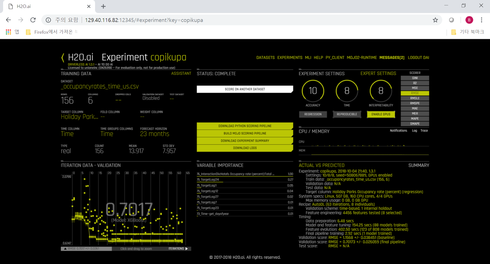
그리고 조종할 부분은 3개의 라디오 다이얼 같은 것 뿐입니다.  왼쪽부터 Accuracy (정확도), Time (시간), Interpretability (기계학습 해석) 다이얼인데, 1~10까지의 '강약'을 조절하는 방식으로 되어 있습니다.   가령 Accuracy를 높일 경우 사용되는 알고리즘이 GLM과 XGBoost에서 XGBoost로 바뀐다든지, Time을 늘릴 경우 training 반복 회수가 12번에서 523번으로 바뀐다든지 하는 식입니다.  어려운 세부 튜닝을 자동으로 해주므로 우리는 그냥 보고서 제출 때까지 시간 여유가 얼마나 있는지 등만 결정하면 되는 것입니다.

물론 아래와 같이 expert setting을 할 수도 있습니다.  Tensorflow라든가 RuleFit 같은 것들은 현재 alpha 버전으로 제공됩니다.

Training을 시작하면 왼쪽 아래에는 validation, 즉 기본적으로 RMSE (Root Mean Square Error)가 display되면서 error가 점차 줄어드는 것을 보실 수 있습니다.  오른쪽 아래에는 data 내의 실제 값과, training 회수가 반복되면서 prediction하는 값의 상관 관계가 그래프로 보여집니다.  처음에는 저 그래프는 분산도가 크게 보여지다가, training이 잘 되면 점차 직선으로 수렴되는 것을 보실 수 있습니다.   또한 중앙 상단의 모델 완성%를 보여주는 계기판 위에는 "3912개의 feature에 대해 896개 모델 중 118개에 대해 평가를 완료"라는 메시지가 보이는데, 이 숫자들은 training이 진행되면서 최적화를 거쳐 계속 동적으로 변화됩니다.

H2O DAI에서는 필요에 따라 띄엄띄엄 GPU를 사용합니다.   다음과 같이 nvidia-smi로도 그 사용 모습을 모니터링할 수 있고, 또 오른쪽 하단의 'GPU usage' tab을 클릭하면 GPU 사용률을 GPU별로 볼 수 있습니다.


Fri Oct  5 00:51:19 2018
+-----------------------------------------------------------------------------+
| NVIDIA-SMI 396.26                 Driver Version: 396.26                    |
|-------------------------------+----------------------+----------------------+
| GPU  Name        Persistence-M| Bus-Id        Disp.A | Volatile Uncorr. ECC |
| Fan  Temp  Perf  Pwr:Usage/Cap|         Memory-Usage | GPU-Util  Compute M. |
|===============================+======================+======================|
|   0  Tesla P100-SXM2...  On   | 00000002:01:00.0 Off |                    0 |
| N/A   31C    P0    39W / 300W |    600MiB / 16280MiB |      0%      Default |
+-------------------------------+----------------------+----------------------+
|   1  Tesla P100-SXM2...  On   | 00000003:01:00.0 Off |                    0 |
| N/A   33C    P0    42W / 300W |    608MiB / 16280MiB |     35%      Default |
+-------------------------------+----------------------+----------------------+
|   2  Tesla P100-SXM2...  On   | 0000000A:01:00.0 Off |                    0 |
| N/A   30C    P0    38W / 300W |    604MiB / 16280MiB |     20%      Default |
+-------------------------------+----------------------+----------------------+
|   3  Tesla P100-SXM2...  On   | 0000000B:01:00.0 Off |                    0 |
| N/A   33C    P0    29W / 300W |     10MiB / 16280MiB |      0%      Default |
+-------------------------------+----------------------+----------------------+

+-----------------------------------------------------------------------------+
| Processes:                                                       GPU Memory |
|  GPU       PID   Type   Process name                             Usage      |
|=============================================================================|
|    0     18750      C   ...uild_cv_model_subprocess-end(prot=True)   295MiB |
|    0     18969      C   ...uild_cv_model_subprocess-end(prot=True)   295MiB |
|    1     18749      C   ...uild_cv_model_subprocess-end(prot=True)   295MiB |
|    1     18970      C   ...el-running(prot=False)-XGBoostModel-fit   303MiB |
|    2     18748      C   ...uild_cv_model_subprocess-end(prot=True)   295MiB |
|    2     18971      C   ...ng(prot=False)-RuleFitModel-fit_glm-fit   299MiB |
+-----------------------------------------------------------------------------+

Training(DAI에서는 Experiment라고 함)이 끝나면 다음과 같이 당장 prediction을 할 수 있는 "Score on another dataset"이라는 메뉴가 제공됩니다.  여기에 training시킨 dataset과 같은 명칭과 종류의 column과 data를 가진 test dataset을 넣으면 아까 정한 target column에 대해 prediction을 해줍니다.   저는 여기에 미리 따로 잘라서 준비해둔 occupancy test dataset을 입력해보았습니다.   그 결과로 다음과 같이 해당 column에 대한 예측값을 CSV로 download 받을 수 있습니다.

이 값을 실제 수치와 비교를 해보면 대략 다음과 같이 나옵니다.  100여줄 정도의 data로 10여분 training한 것치고는 괜찮은 예측치입니다.

또한, 이런 예측을 이렇게 DAI 서버의 web interface 말고, 여기서 train된 모델을 다른 서버로 옮겨서 python 혹은 java client program을 거쳐서 수행할 수도 있습니다.  이에 대해서는 다른 posting에서 다루겠습니다.