2018년 10월 25일 목요일

GPUdb인 Kinetica와 Postgresql의 대결

Kinetica는 GPU를 이용한 in-memory DB로서, 주로 OLTP용보다는 OLAP용으로 사용됩니다.    아래에 간단한 TPC-H data와 query를 이용하여 일반 DBMS(여기서는 postgresql)와의 성능 비교 및 그때 CPU-GPU간의 NVLink가 어떤 효과를 내는지 nvprof로 분석해보았습니다.   아래 test는 모두 POWER9 + V100 GPU의 IBM AC922 서버로 진행했습니다.

Postgresql과 Kinetica 모두 TPC-H에서 제공되는 dbgen으로 생성한 data를 사용했습니다.  여기서 DB 크기는 10GB로 했습니다.  이렇게 하면 delimeter가 '|'로 되어 있는 SAM file들이 만들어지는데, 실제로 DB에 load를 하려면 맨 끝에 붙은 '|'은 제거해야 하더군요.

[root@localhost dbgen]# nohup ./dbgen -s 10 &

[root@localhost dbgen]# ls -ltr *.tbl
-rw-r--r--. 1 root root   14176368 Oct 23 09:35 supplier.tbl
-rw-r--r--. 1 root root        389 Oct 23 09:35 region.tbl
-rw-r--r--. 1 root root  243336157 Oct 23 09:35 part.tbl
-rw-r--r--. 1 root root 1204850769 Oct 23 09:35 partsupp.tbl
-rw-r--r--. 1 root root 1749195031 Oct 23 09:35 orders.tbl
-rw-r--r--. 1 root root       2224 Oct 23 09:35 nation.tbl
-rw-r--r--. 1 root root 7775727688 Oct 23 09:35 lineitem.tbl
-rw-r--r--. 1 root root  244847642 Oct 23 09:35 customer.tbl

Postgres에서는 다음과 같이 dbgen에 포함된 dss.ddl script를 이용하여 필요한 table들을 생성했습니다.

[root@localhost dbgen]# su - postgres
Last login: Mon Oct 22 17:27:48 KST 2018 on pts/1

-bash-4.2$ createdb dss
-bash-4.2$ psql dss
psql (9.2.23)
Type "help" for help.

dss=# \i /home/data/2.17.3/dbgen/dss.ddl

dss=# \d ORDERS
                Table "public.orders"
     Column      |         Type          | Modifiers
-----------------+-----------------------+-----------
 o_orderkey      | integer               | not null
 o_custkey       | integer               | not null
 o_orderstatus   | character(1)          | not null
 o_totalprice    | numeric(15,2)         | not null
 o_orderdate     | date                  | not null
 o_orderpriority | character(15)         | not null
 o_clerk         | character(15)         | not null
 o_shippriority  | integer               | not null
 o_comment       | character varying(79) | not null

그 다음에 다음과 같이 SAM file에서 postgresql table 안으로 loading을 합니다.  아래는 LINEITEM의 table 예만 들었습니다.

dss=# copy lineitem from '/home/data/2.17.3/dbgen/lineitem.csv' with (FORMAT csv, DELIMITER '|');
COPY 59986052


Kinetica에도 이 SAM file을 만들고 load 하기 위해서는 다음과 같은 menu를 이용하면 됩니다.   다만 Kinetica는 GPU를 이용한 분산 DB이기 때문에, shard key를 지정하는 등 추가적인 설정 과정을 거쳐야 합니다.  (여기서는 상세히 표시하지 않았습니다.  저도 제가 직접 못하고 저희 파트너사인 Unione INC의 엔지니어 도움을 받았습니다.)


먼저, TPC-H의 query들 중 1개씩의 query를 수행해보겠습니다.  이 query는 join 등이 그렇게까지 크지 않은 query라서 GPUdb가 일반 RDBMS에 비해 그다지 더 유리하지도 않은 query입니다.  그런데도, 또 별다른 tuning 없이도, Kinetica가 20배 정도 빠른 것을 보실 수 있습니다.  모두 2번씩 돌린 것이므로, postgresql에서도 data는 이미 memory에 cache된 상태라서 disk 병목은 전혀 없다고 보셔도 됩니다.

-bash-4.2$ time psql -d dss -f /home/data/RunQuery/q16.sql > /tmp/ooo

real    1m1.267s
user    0m0.374s
sys     0m0.000s

[root@localhost ~]# time /opt/gpudb/bin/kisql -host 127.0.0.1 -f /home/data/RunQuery/q16.sql > /tmp/iii

real    0m3.046s
user    0m3.729s
sys     0m0.770s

특히 Kinetica의 경우는 아래처럼 query 결과에 Query Execution Time과 Data Transfer Time을 각각 명기합니다.   GPUdb에서는 query execution보다 data를 transfer하는데 더 많은 시간이 걸린다는 것을 보실 수 있습니다.  이런 것 때문에 특히 CPU와 GPU간의 연결이 CPU냐 GPU냐가 매우 중요합니다.

| Brand#54   | ECONOMY PLATED BRASS        |       14 |              4 |
| Brand#55   | STANDARD BURNISHED BRASS    |       14 |              4 |
+------------+-----------------------------+----------+----------------+
Rows read = 27840
Query Execution Time: 0.495 s
Data Transfer Time: 2.283 s


이 시스템에 CPU core는 32개나 있지만 GPU는 딱 2장 뿐입니다.  이럴 경우 저런 query를 10개씩 병렬로 수행하면 CPU가 더 빠를 수도 있지 않을까요 ?  꼭 그렇지는 않습니다.

여기서는 TPC-H의 16번과 19번 query 2개를 5번씩, 총 10개를 한꺼번에 수행하는 방식으로 돌리겠습니다.

Postgres에서 돌릴 script는 다음과 같습니다.

-bash-4.2$ cat 1.sh
date
echo "Starting"
psql -d dss -f /home/data/RunQuery/q16.sql &
psql -d dss -f /home/data/RunQuery/q19.sql &
...(총 10줄)
wait
date
echo "Finished"

Kinetica에서 돌릴 script도 사실상 똑같은 내용입니다.

[root@localhost ~]# cat /tmp/1.sh
date
echo "Starting"
/opt/gpudb/bin/kisql -host 127.0.0.1 -f /home/data/RunQuery/q16.sql &
/opt/gpudb/bin/kisql -host 127.0.0.1 -f /home/data/RunQuery/q19.sql &
/opt/gpudb/bin/kisql -host 127.0.0.1 -f /home/data/RunQuery/q16.sql &
/opt/gpudb/bin/kisql -host 127.0.0.1 -f /home/data/RunQuery/q19.sql &
...  (총 10줄)
wait
date
echo "Finished"


각각의 수행 결과는 다음과 같습니다.   Kinetica도 GPU가 2장 뿐인 환경에서도 10개의 동시 query를 잘 수행해내며, 여전히 6배 정도 빠릅니다.

Postgresql는 다음과 같습니다.

-bash-4.2$ time ./1.sh > p.txt 

real    1m6.947s
user    0m1.891s
sys     0m0.055s

Kinetica는 다음과 같습니다.

[root@localhost ~]# time /tmp/1.sh > /tmp/k.txt   

real    0m8.545s
user    0m29.965s
sys     0m20.525s


Kinetica에서 이 query를 처리하기 전에, nvprof를 이용해 profile data를 받기 위해서 Kinetica의 구동 script 중 일부를 수정한 뒤 restart 해주어야 합니다.  수정은 다음과 같이 간단합니다.  아래 붉은 색 부분의 명령어를 삽입해주기만 하면 됩니다.

[root@localhost ~]# vi /opt/gpudb/core/bin/gpudb
...
#    nohup $HOST_MANAGER_CMD >> $HOST_MANAGER_LOG_FILENAME 2>&1 &
    nohup /usr/local/cuda-9.2/bin/nvprof --log-file /tmp/nvprof/%p.txt --export-profile /tmp/nvprof/%p.nvvp --print-gpu-trace --profile-child-processes $HOST_MANAGER_CMD >> $HOST_MANAGER_LOG_FILENAME 2>&1 &
...


이렇게 얻은 profile data를 분석해보면, GPUdb의 대표적인병목인 cuda memcpy HtoD (CPU to GPU) 및 DtoH (GPU to CPU)의 사용되는 대역폭을 보실 수 있습니다.   대략 35GB/sec에 달합니다.   참고로, POWER9과 V100 GPU 사이를 연결하는 NVLink는 3개의 port를 aggregate시킨 것이라서, 이론상 단방향 대역폭이 75GB/sec (양방향 150GB/sec)에 달합니다.  PCIe Gen3 버스의 이론상 단방향 대역폭이 16GB/sec(양방향 32GB/sec)에 불과하다는 것을 생각하면, Kinetica와 같은 GPUdb를 사용할 경우 CPU와 GPU의 연결은 반드시 NVLink가 되어야 한다는 것을 쉽게 아실 수 있습니다.

2018년 10월 15일 월요일

Python Image Library(PIL, Pillow)의 성능 테스트

Python Image Library (PIL, python3에서는 pillow)을 이용하여 python에서 image 생성/변경 등이 가능합니다.  그리고, 이 성능 평가를 위해서는 pillow-perf라는 code를 이용할 수 있습니다.   먼저 pillow-perf를 git으로부터 clone 합니다.

[root@python1 ~]# git clone https://github.com/python-pillow/pillow-perf.git

아래와 같이 pip로 필요 package들을 설치합니다.

[root@python1 ~]# cd pillow-perf/testsuite/

[root@python1 testsuite]# pip install -r ./requirements.txt

이제 다음과 같이 몇가지 테스트를 수행해봅니다.   아래의 결과는 Naver nCloud에서 제공되는 E5-2660 v4@2.00GHz에서 수행된 것입니다.  이 테스트는 single-thread로 되어 있고, IBM POWER8/POWER9에서도 동일한 방법으로 수행할 수 있습니다.

[root@python1 testsuite]#  ./run.py scale --progress

Scale 2560×1600 RGB image
    to 26x16 bil        0.01323 s   309.62 Mpx/s
    to 26x16 bic        0.02488 s   164.62 Mpx/s
    to 26x16 lzs        0.03783 s   108.28 Mpx/s
    to 320x200 bil      0.02107 s   194.43 Mpx/s
    to 320x200 bic      0.03579 s   114.45 Mpx/s
    to 320x200 lzs      0.05393 s    75.95 Mpx/s
    to 2048x1280 bil    0.05956 s    68.77 Mpx/s
    to 2048x1280 bic    0.08711 s    47.02 Mpx/s
    to 2048x1280 lzs    0.12037 s    34.03 Mpx/s
    to 5478x3424 bil    0.28072 s    14.59 Mpx/s
    to 5478x3424 bic    0.38422 s    10.66 Mpx/s
    to 5478x3424 lzs    0.49239 s     8.32 Mpx/s

[root@python1 testsuite]# ./run.py scale --mode RGBA

Scale 2560×1600 RGBA image
    to 26x16 bil        0.02508 s   163.33 Mpx/s
    to 26x16 bic        0.04012 s   102.09 Mpx/s
    to 26x16 lzs        0.05564 s    73.62 Mpx/s
    to 320x200 bil      0.03434 s   119.29 Mpx/s
    to 320x200 bic      0.04993 s    82.04 Mpx/s
    to 320x200 lzs      0.07300 s    56.11 Mpx/s
    to 2048x1280 bil    0.10238 s    40.01 Mpx/s
    to 2048x1280 bic    0.13699 s    29.90 Mpx/s
    to 2048x1280 lzs    0.18249 s    22.44 Mpx/s
    to 5478x3424 bil    0.51842 s     7.90 Mpx/s
    to 5478x3424 bic    0.63934 s     6.41 Mpx/s
    to 5478x3424 lzs    0.78471 s     5.22 Mpx/s

[root@python1 testsuite]# ./run.py scale --runs 50

Scale 2560×1600 RGB image
    to 26x16 bil        0.01308 s   313.08 Mpx/s
    to 26x16 bic        0.02493 s   164.28 Mpx/s
    to 26x16 lzs        0.03770 s   108.64 Mpx/s
    to 320x200 bil      0.02115 s   193.62 Mpx/s
    to 320x200 bic      0.03549 s   115.42 Mpx/s
    to 320x200 lzs      0.05399 s    75.87 Mpx/s
    to 2048x1280 bil    0.05944 s    68.91 Mpx/s
    to 2048x1280 bic    0.08735 s    46.89 Mpx/s
    to 2048x1280 lzs    0.12058 s    33.97 Mpx/s
    to 5478x3424 bil    0.28272 s    14.49 Mpx/s
    to 5478x3424 bic    0.38564 s    10.62 Mpx/s
    to 5478x3424 lzs    0.49298 s     8.31 Mpx/s

[root@python1 testsuite]# ./run.py blur

Blur 2560×1600 RGB image
    1px                 0.22742 s    18.01 Mpx/s
    10px                0.22500 s    18.20 Mpx/s
    30px                0.22543 s    18.17 Mpx/s

[root@python1 testsuite]# ./run.py convert

Convert 2560×1600 RGB image
    RGB to L            0.00539 s   760.07 Mpx/s
    RGBA to LA          0.00652 s   627.90 Mpx/s
    RGBa to RGBA        0.03590 s   114.08 Mpx/s
    RGBA to RGBa        0.00851 s   481.57 Mpx/s


그 외에, 실제 jpg 파일들을 이용하여 몇가지 PIL 처리를 하는 sample code를 수행해보는 것도 괜찮습니다.

[root@python1 ~]# cat piljpg.py
from PIL import Image, ImageFilter
list = [ "1.jpg", "2.jpg", "3.jpg", "4.jpg", "5.jpg", "6.jpg", "7.jpg", "8.jpg", "9.jpg", "10.jpg" ]
for x in list:
    im = Image.open(x)
    print(im.size)
    im.save('pasta.jpg')
    im = Image.open(x)
    size = (64, 64)
    im.thumbnail(size)
    im.save('python-thumb.jpg')
    im = Image.open(x)
    cropImage = im.crop((100, 100, 150, 150))
    cropImage.save('python-crop.png')
    im = Image.open(x)
    img2 = im.resize((600, 600))
    img2.save('python-600.jpg')
    img3 = im.rotate(90)
    img3.save('rotate.jpg')
    im = Image.open(x)
    blurImage = im.filter(ImageFilter.BLUR)
    blurImage.save('python-blur.jpg')


[root@python1 ~]# time python piljpg.py
(2281, 3072)
(972, 1422)
(972, 1422)
(972, 1422)
(972, 1422)
(972, 1422)
(5040, 4912)
(1600, 1280)
(2281, 3072)
(972, 1422)

real    0m15.047s
user    0m14.759s
sys     0m0.285s


piljpg.py의 코드와 거기에 쓰인 *.jpg 파일은 아래 구글 드라이브에 올려놓았습니다.

https://drive.google.com/open?id=1LdjcDXrQ3Dps0ertGwGMyMYKRhxo5FEB

2018년 10월 11일 목요일

Python을 위한 local private repository 만들기 (bandersnatch + nginx)

Python은 그 특성상 필요에 따라 자주 새로운 package를 설치해서 써야 하는데, 이를 위해서는 해당 서버가 443번 포트를 통해 인터넷에 연결되어 있는 환경이어야 합니다.  그러나 실제로는 대부분의 기업용 data center들에서는 인터넷과의 연결이 완전히 단절되어 있으므로 python을 쓰기에 매우 불편합니다.   이는 x86이든 ppc64le이든 arm이든 모든 CPU 아키텍처에서 공통적으로 골치아파하는 문제이며, 국내 대기업들은 물론 해외 유명 인터넷 업체에서도 다 공통적으로 겪는 문제입니다.  가령 Pillow라는 package를 import해서 쓰려면 먼저 그 package를 설치해야 하는데, pip 명령으로 설치하면 아래처럼 그때그때 인터넷에서 source를 download 받아서 즉석에서 build해서 설치합니다.


[bsyu@p57a22 ~]$ pip install Pillow
Collecting Pillow
  Downloading https://files.pythonhosted.org/packages/1b/e1/1118d60e9946e4e77872b69c58bc2f28448ec02c99a2ce456cd1a272c5fd/Pillow-5.3.0.tar.gz (15.6MB)
    100% |████████████████████████████████| 15.6MB 11.6MB/s
Building wheels for collected packages: Pillow
  Running setup.py bdist_wheel for Pillow ... done
  Stored in directory: /home/bsyu/.cache/pip/wheels/df/81/28/47e761b5e307472ba7c2c5ced6e52037bbefe33c9c4b2a627e
Successfully built Pillow
Installing collected packages: Pillow
Successfully installed Pillow-5.3.0


이런 문제를 해결하는 왕도는 따로 없으나, 가장 근본적인 해결책은 외부망과 분리된 data center 내에 python을 위한 private local repository를 구성하는 것입니다.   다만 여기에는 2가지 문제가 있습니다.

1) Public python repository는 pypi.org (실제로는 files.pythonhosted.org) 인데, 전체 repository 크기가 800GB가 넘고, 날마다 계속 커지고 있습니다.

2) 기존 python package들의 새버전과, 또 아예 새로 만들어지는 python package들이 날마다 쏟아져 나오므로 주기적으로 자주 update를 해줘야 합니다.

보통 1번 문제는 (돈 있는 기업들 입장에서는) 큰 문제가 아닙니다.  Local repository server에 넉넉한 크기의 disk를 쓰면 되기 때문입니다.   문제는 2번 문제인데, 이것도 뾰족한 방법은 없고 외부에서 (1달에 1번 정도) 주기적으로 pypi.org의 내용을 backup 받아서 USB 외장 disk에 담아 data center로 들여온 뒤 local repository server에 부어주는 수 밖에 없습니다.

이런 정책만 정해지면 local repository server를 구성하는 것은 그다지 어렵지 않습니다.    다음과 같이 bandersnatch라는 package를 이용하면 쉽습니다.

아래의 모든 테스트는 ppc64le 아키텍처인 IBM POWER8 processor와 Redhat 7.5를 이용해서 수행되었습니다.  혹자는 x86_64를 위한 python repository는 어디 있는지 알겠는데 ppc64le를 위한 것은 어디 있냐고 여쭈시는 분도 있습니다만,  x86이나 ppc64le나 aarch64나 모두 같은 repository를 사용합니다. 


먼저, 다음과 같이 Anaconda3가 설치된 환경에서 pip로 bandersnatch를 설치합니다. 

[bsyu@p57a22 ~]$ which pip
~/anaconda3/bin/pip

[bsyu@p57a22 ~]$ pip install -r https://bitbucket.org/pypa/bandersnatch/raw/stable/requirements.txt
...
Successfully installed apipkg-1.4 bandersnatch-2.0.0 coverage-4.3.1 execnet-1.4.1 mock-2.0.0 packaging-16.8 pbr-1.10.0 pep8-1.7.0 py-1.4.32 pyflakes-1.3.0 pyparsing-2.1.10 pytest-3.0.5 pytest-cache-1.0 pytest-catchlog-1.2.2 pytest-codecheckers-0.2 pytest-cov-2.4.0 pytest-timeout-1.2.0 python-dateutil-2.6.0 requests-2.12.4 setuptools-33.1.1 six-1.10.0 xmlrpc2-0.3.1

[bsyu@p57a22 ~]$ which bandersnatch
~/anaconda3/bin/bandersnatch

그리고 'bandersnatch mirror' 명령을 수행합니다.   그러면 기본 /etc/bandersnatch.conf을 만들어줍니다.  이 때문에 이 명령은 일단 sudo 권한이 필요합니다.

[bsyu@p57a22 ~]$ sudo /home/bsyu/anaconda3/bin/bandersnatch mirror
2018-10-10 03:31:32,069 WARNING: Config file '/etc/bandersnatch.conf' missing, creating default config.
2018-10-10 03:31:32,069 WARNING: Please review the config file, then run 'bandersnatch' again.

이 /etc/bandersnatch.conf를 필요에 따라 수정합니다.  여기서는 어느 directory에 python repository를 내려받을 것인지만 수정했습니다.

[bsyu@p57a22 ~]$ sudo vi /etc/bandersnatch.conf
...
; directory = /srv/pypi
directory = /home/bsyu/files/pypi
...

다시 'bandersnatch mirror' 명령을 수행하면 정규 public repository (files.pythonhosted.org)를 통째로 download 받습니다.   800GB가 넘는다는 점에 유의하시기 바랍니다.  저도 끝까지 download 받아본 적은 없고, disk가 부족하여 도중에 끊어야 했습니다.

[bsyu@p57a22 ~]$ bandersnatch mirror
2018-10-10 03:33:35,064 INFO: bandersnatch/2.0.0 (cpython 3.7.0-final0, Linux ppc64le)
2018-10-10 03:33:35,064 INFO: Setting up mirror directory: /home/bsyu/files/pypi/
2018-10-10 03:33:35,064 INFO: Setting up mirror directory: /home/bsyu/files/pypi/web/simple
2018-10-10 03:33:35,064 INFO: Setting up mirror directory: /home/bsyu/files/pypi/web/packages
2018-10-10 03:33:35,064 INFO: Setting up mirror directory: /home/bsyu/files/pypi/web/local-stats/days
2018-10-10 03:33:35,064 INFO: Generation file missing. Reinitialising status files.
2018-10-10 03:33:35,065 INFO: Status file missing. Starting over.
2018-10-10 03:33:35,065 INFO: Syncing with https://pypi.python.org.
2018-10-10 03:33:35,065 INFO: Current mirror serial: 0
2018-10-10 03:33:35,065 INFO: Syncing all packages.
2018-10-10 03:33:37,934 INFO: Trying to reach serial: 4358961
2018-10-10 03:33:37,934 INFO: 154638 packages to sync.
...
2018-10-10 03:53:50,360 INFO: Downloading: https://files.pythonhosted.org/packages/8a/5c/625ac1a93da3a672f52d947023770331b958a1100cd9889b727cde5f7ba5/CommonMark-0.7.5-py2.py3-none-any.whl
2018-10-10 03:53:50,360 DEBUG: Getting https://files.pythonhosted.org/packages/8a/5c/625ac1a93da3a672f52d947023770331b958a1100cd9889b727cde5f7ba5/CommonMark-0.7.5-py2.py3-none-any.whl (serial None)
2018-10-10 03:53:50,363 INFO: Syncing package: CompCamps-Cash-Api (serial 4042164)
2018-10-10 03:53:50,363 DEBUG: Getting /pypi/CompCamps-Cash-Api/json (serial 4042164)
2018-10-10 03:53:50,370 INFO: Downloading: https://files.pythonhosted.org/packages/77/16/44a297228a439484d049cdad818c7f6691c162b4cd741c619caeb208bb1e/CommonMark-0.7.5.tar.gz
2018-10-10 03:53:50,371 DEBUG: Getting https://files.pythonhosted.org/packages/77/16/44a297228a439484d049cdad818c7f6691c162b4cd741c619caeb208bb1e/CommonMark-0.7.5.tar.gz (serial None)
...

이제 해당 directory에 가보면 다음과 같이 web/packages 밑에 실제 python package 파일들이 download 되어진 것을 보실 수 있습니다.   web/simple은 그 파일들에 대한 index directory입니다.

[bsyu@p57a22 ~]$ cd files/pypi

[bsyu@p57a22 pypi]$ ls
generation  todo  web

[bsyu@p57a22 pypi]$ cd web

[bsyu@p57a22 web]$ ls
local-stats  packages  simple

[bsyu@p57a22 web]$ cd packages/

[bsyu@p57a22 packages]$ ls
00  0b  16  21  2c  37  42  4e  59  64  6f  7a  85  90  9b  a6  b1  bc  c7  d2  dd  e8  f3  fe
01  0c  17  22  2d  38  43  4f  5a  65  70  7b  86  91  9c  a7  b2  bd  c8  d3  de  e9  f4  ff
02  0d  18  23  2e  39  44  50  5b  66  71  7c  87  92  9d  a8  b3  be  c9  d4  df  ea  f5
03  0e  19  24  2f  3a  45  51  5c  67  72  7d  88  93  9e  a9  b4  bf  ca  d5  e0  eb  f6
04  0f  1a  25  30  3b  46  52  5d  68  73  7e  89  94  9f  aa  b5  c0  cb  d6  e1  ec  f7
05  10  1b  26  31  3c  47  53  5e  69  74  7f  8a  95  a0  ab  b6  c1  cc  d7  e2  ed  f8
06  11  1c  27  32  3d  49  54  5f  6a  75  80  8b  96  a1  ac  b7  c2  cd  d8  e3  ee  f9
07  12  1d  28  33  3e  4a  55  60  6b  76  81  8c  97  a2  ad  b8  c3  ce  d9  e4  ef  fa
08  13  1e  29  34  3f  4b  56  61  6c  77  82  8d  98  a3  ae  b9  c4  cf  da  e5  f0  fb
09  14  1f  2a  35  40  4c  57  62  6d  78  83  8e  99  a4  af  ba  c5  d0  db  e6  f1  fc
0a  15  20  2b  36  41  4d  58  63  6e  79  84  8f  9a  a5  b0  bb  c6  d1  dc  e7  f2  fd


이렇게 download된 generation todo web의 3개 directory를 포함하는 python repository directory 전체 (여기서는 /home/bsyu/files/pypi)를 USB 외장 disk 등에 복사하여 local repository로 사용할 서버에 옮깁니다.   여기서는 편의상 그냥 download 받은 서버에서 직접 local repository 서버를 구성하겠습니다.

https을 통해서 다른 서버들에게 python repository 서비스를 하기 위해서는 당연히 web 서버를 구성해야 합니다.  여기서는 간단하게 nginx를 사용하겠습니다.  먼저 nginx를 YUM 명령으로 설치한 뒤, /etc/nginx/nginx.conf를 수정합니다.  단, 여기서 http(80번 포트)가 아닌 https(443번 포트)를 구성해야 합니다.  그리고 root를 복사한 directory 중 'web' directory로 정해야 하고, SSL certificate과 그 key도 등록해야 합니다.   server_name은 FQDN(Fully Qualified Domain Name)으로 합니다.  여기서는 IP address로 했습니다.

[bsyu@p57a22 ~]$ sudo yum install nginx

[bsyu@p57a22 ~]$ sudo vi /etc/nginx/nginx.conf
...
    server {
        listen       443 ssl http2 default_server;
        listen       [::]:443 ssl http2 default_server;
#        root         /usr/share/nginx/html;
        root         /home/bsyu/files/pypi/web;
        autoindex on;
        charset utf-8;

#        server_name  _;
        server_name  129.40.xx.xx;
        ssl_certificate "/etc/pki/nginx/private/domain.crt";
        ssl_certificate_key "/etc/pki/nginx/private/domain.key";
        ssl_session_cache shared:SSL:1m;
        ssl_session_timeout  10m;
...

이제 SSL 구성을 위해 crt와 key를 생성합니다.  여기서는 1년간 유효한 Self-Signed Certificate (x509)를 만들었습니다.

[bsyu@p57a22 ~]$ cd /etc/pki/nginx/private

[root@p57a22 private]# openssl req -newkey rsa:2048 -nodes -keyout domain.key -x509 -days 365 -out domain.crt
Generating a 2048 bit RSA private key
.......................................................................................+++++
..............................+++++
writing new private key to 'domain.key'
-----
You are about to be asked to enter information that will be incorporated
into your certificate request.
What you are about to enter is what is called a Distinguished Name or a DN.
There are quite a few fields but you can leave some blank
For some fields there will be a default value,
If you enter '.', the field will be left blank.
-----
Country Name (2 letter code) [AU]:.
State or Province Name (full name) [Some-State]:.
Locality Name (eg, city) []:.
Organization Name (eg, company) [Internet Widgits Pty Ltd]:.
Organizational Unit Name (eg, section) []:.
Common Name (e.g. server FQDN or YOUR name) []:129.40.xx.xx
Email Address []:.

[root@p57a22 private]# ls -ltr
total 8
-rw-r--r-- 1 root root 1704 Oct 11 00:13 domain.key
-rw-r--r-- 1 root root 1107 Oct 11 00:13 domain.crt

생성된 certificate과 key의 검사는 아래와 같이 할 수 있습니다. 

[root@p57a22 private]# openssl x509 -text -noout -in domain.crt
Certificate:
    Data:
        Version: 3 (0x2)
        Serial Number:
            a7:03:d9:7b:33:2d:53:7c
    Signature Algorithm: sha256WithRSAEncryption
        Issuer: CN=129.40.xx.xx
        Validity
            Not Before: Oct 11 04:13:00 2018 GMT
            Not After : Oct 11 04:13:00 2019 GMT
        Subject: CN=129.40.116.82
        Subject Public Key Info:
            Public Key Algorithm: rsaEncryption
                Public-Key: (2048 bit)
                Modulus:
                    00:ca:73:3c:7f:e6:29:1e:5e:7b:ff:b5:98:30:ce:
                    fb:48:0e:bc:96:fd:5b:7f:1e:23:e5:62:8f:74:8e:
 ...

[root@p57a22 private]# openssl rsa -check -in domain.key
RSA key ok
writing RSA key
-----BEGIN RSA PRIVATE KEY-----
MIIEpAIBAAKCAQEAynM8f+YpHl57/7WYMM77SA68lv1bfx4j5WKPdI6ftW2lRdrw
fUikVx0C+2ni3QB6y/xuT8yT0eiCPT5Ak4yGpDSsfcfzDOFgVSB02irWmX/KUNIS
/zS+E7SkAfariUEFa8iRjt2kmDpi65YGKH9NY7p136NcZOSZQx2wsAU0UM5Pjtci
....

이제 생성된 certificate과 key를 합해 PEM을 만듭니다. 

[root@p57a22 private]# cat domain.crt domain.key >> domain.pem

이제 nginx를 start 합니다.

[root@p57a22 private]# systemctl status nginx

그리고 pip에서 이 129.40.xx.xx를 trusted-host로 사용하도록 ~/.pip/pip.conf를 생성하여 다음과 같은 내용을 넣어줍니다.

[bsyu@p57a22 ~]$ vi .pip/pip.conf
[global]
trusted-host = 129.40.xx.xx
index = https://129.40.xx.xx:443/packages
index-url = https://129.40.xx.xx:443/simple
cert = /etc/pki/nginx/private/domain.pem

이제 CommonMark라는 package를 설치해봅니다.   기존처럼 files.pythonhosted.org가 아니라 129.40.xx.xx에서 package source를 가져오는 것을 보실 수 있습니다.

[bsyu@p57a22 ~]$ pip install CommonMark
Looking in indexes: https://129.40.xx.xx:443/simple
Collecting CommonMark
  Downloading https://129.40.xx.xx:443/packages/ab/ca/439c88039583a29564a0043186875258e9a4f041fb5c422cd387b8e10175/commonmark-0.8.1-py2.py3-none-any.whl (47kB)
    100% |████████████████████████████████| 51kB 37.8MB/s
Requirement already satisfied: future in ./anaconda3/lib/python3.7/site-packages (from CommonMark) (0.16.0)
Installing collected packages: CommonMark
Successfully installed CommonMark-0.8.1

2018년 10월 5일 금요일

IBM이 자랑하는 POWER9 + V100 GPU의 조합이 H2O DriverlessAI에 어떤 도움이 될까 ?

H2O Driverless AI는 model training 중 GPU에서 돌리는 것이 더 효과적이라고 판단될 때마다 필요에 따라 드문드문 GPU를 사용합니다.   이는 우측 하단의 "GPU usage" tab을 클릭하면 아래와 같이 보실 수 있습니다.


물론 nvidia-smi 에서도 모니터링하실 수 있습니다.   GPU 1개당 1개의 process가 수행되는 것이 아니라, GPU 메모리가 허용하는 한 필요에 따라 GPU 1개당 여러 개의 process들이 수행되기도 합니다.

Fri Oct  5 03:36:45 2018
+-----------------------------------------------------------------------------+
| NVIDIA-SMI 396.26                 Driver Version: 396.26                    |
|-------------------------------+----------------------+----------------------+
| GPU  Name        Persistence-M| Bus-Id        Disp.A | Volatile Uncorr. ECC |
| Fan  Temp  Perf  Pwr:Usage/Cap|         Memory-Usage | GPU-Util  Compute M. |
|===============================+======================+======================|
|   0  Tesla P100-SXM2...  On   | 00000002:01:00.0 Off |                    0 |
| N/A   34C    P0    64W / 300W |    455MiB / 16280MiB |     40%      Default |
+-------------------------------+----------------------+----------------------+
|   1  Tesla P100-SXM2...  On   | 00000003:01:00.0 Off |                    0 |
| N/A   36C    P0    77W / 300W |    455MiB / 16280MiB |     38%      Default |
+-------------------------------+----------------------+----------------------+
|   2  Tesla P100-SXM2...  On   | 0000000A:01:00.0 Off |                    0 |
| N/A   32C    P0    71W / 300W |    455MiB / 16280MiB |     40%      Default |
+-------------------------------+----------------------+----------------------+
|   3  Tesla P100-SXM2...  On   | 0000000B:01:00.0 Off |                    0 |
| N/A   36C    P0    64W / 300W |    455MiB / 16280MiB |     38%      Default |
+-------------------------------+----------------------+----------------------+

+-----------------------------------------------------------------------------+
| Processes:                                                       GPU Memory |
|  GPU       PID   Type   Process name                             Usage      |
|=============================================================================|
|    0     94004      C   ...el-running(prot=False)-XGBoostModel-fit   445MiB |
|    1     94011      C   ...el-running(prot=False)-XGBoostModel-fit   445MiB |
|    2     94044      C   ...el-running(prot=False)-XGBoostModel-fit   445MiB |
|    3     94126      C   ...el-running(prot=False)-XGBoostModel-fit   445MiB |
+-----------------------------------------------------------------------------+


과연 여기서 NVLink가 어느 정도의 효과를 발휘할까요 ?  그것을 확인하는 가장 쉽고 생생한 방법은 nvprof 명령을 이용하여 DriverlessAI process들이 GPU를 어떻게 사용하는지 profile을 떠보는 것입니다.

먼저, DAI의 홈 디렉토리에 있는 start-dai.sh를 다음과 같이 수정합니다.  원래의 line은 #으로 막아놓았고, 아래 붉은색의 명령어들이 새로 삽입된 nvprof 명령어입니다.

[root@p57a22 dai-1.3.1-linux-ppc64le]# cat start-dai.sh
#!/bin/bash

if [ "x${RUN_DAI_CREATE_PIDFILE}" == "x1" ]; then
# python -m h2oai &
 /usr/local/cuda-9.2/bin/nvprof --log-file /tmp/nvprof1.%p.txt --export-profile /tmp/nvprof1.%p.nvvp --print-gpu-trace --profile-child-processes python -m h2oai &
    echo $! > ${RUN_DAI_PIDFILE_DIR}/dai.pid
else
# exec python -m h2oai
    exec /usr/local/cuda-9.2/bin/nvprof --log-file /tmp/nvprof1.%p.txt --export-profile /tmp/nvprof1.%p.nvvp --print-gpu-trace --profile-child-processes python -m h2oai
fi


위와 같이 해놓고 kill-dai.sh를 수행하여 기존 DAI를 stop시킨 뒤, run-dai.sh를 수행하여 DAI를 새로 구동한 뒤에 큼직한 dataset으로 training을 해봅니다.   이때, 다음과 같이 child process마다 txt와 nvvp로 텍스트와 바이너리 로그 파일이 생성되는 것을 보실 수 있습니다.

[root@p57a22 dai-1.3.1-linux-ppc64le]# ls -l /tmp/nvprof1*
...
-rw-r--r-- 1 root root 170096640 Oct  5 03:16 /tmp/nvprof1.83368.nvvp
-rw-r--r-- 1 root root 233180816 Oct  5 03:22 /tmp/nvprof1.83368.txt
-rw-r--r-- 1 root root 180073472 Oct  5 03:16 /tmp/nvprof1.83405.nvvp
-rw-r--r-- 1 root root 246428557 Oct  5 03:20 /tmp/nvprof1.83405.txt
...

이 중 하나를 CUDA에 딸려 있는 NVIDIA Visual Profiler (NVVP)로 분석해보면 다음과 같습니다.


"CUDA memcpy HtoD" (Host to Device, 즉 서버 CPU에서 GPU로의 memcpy도 9 GB/s에 가깝고 DtoD (GPU간의 memcpy)는 134 GB/s에 가깝게 사용되는 것을 보실 수 있습니다.

특히 8개의 GPU를 장착한 일반 x86 기반 GPU 서버들은 NVLink를 1개씩만 이용하여 연결되므로 GPU간의 통신은 이론상 50 GB/s, CPU와 GPU간의 통신은 이론상 32 GB/s가 최대인 것에 비해, IBM AC922은 3개의 NVLink를 aggregation시켜 CPU와 GPU이나 GPU끼리나 모두 150 GB/s로 연결된 것이 H2O DriverlessAI의 운용에 크게 유리하다는 것을 쉽게 보실 수 있습니다.


H2O DriverlessAI에서 제공하는 python client program 수행

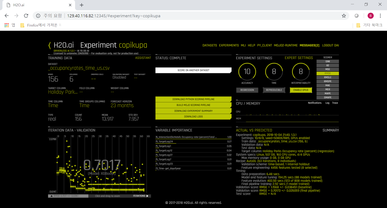
H2O DAI는 training한 모델을 이용하는 client program을 python 혹은 MOJO(java) 형태로 제공해줍니다.  먼저번 posting에서 train된 모델에 대한 python client program을 download 받기 위해서는 "Download python scoring pipeline"이라는 메뉴를 click하면 됩니다.   scoring.zip이라는 zip 파일을 web browser로 download 받을 수 있습니다. 


서버 상에서는 이 파일은 다음과 같이 임시 directory에 생성되어 있으니 그걸 download 받아서 사용해도 됩니다.

[root@p57a22 dai-1.3.1-linux-ppc64le]# ls -l ./tmp/h2oai_experiment_copikupa/scoring_pipeline/scorer.zip
-rw-rw----+ 1 root root 95622433 Oct  4 21:40 ./tmp/h2oai_experiment_copikupa/scoring_pipeline/scorer.zip

[root@p57a22 dai-1.3.1-linux-ppc64le]# cp ./tmp/h2oai_experiment_copikupa/scoring_pipeline/scorer.zip /home/data

이것의 압축을 풀면 다음과 같이 train된 model을 포함하는 wheel 파일과 함께, python client program을 구성하는 python code 및 shell program들이 들어 있습니다.

[root@p57a22 data]# unzip scorer.zip
Archive:  scorer.zip
   creating: scoring-pipeline/
  inflating: scoring-pipeline/scoring.thrift
  inflating: scoring-pipeline/requirements.txt
  inflating: scoring-pipeline/environment.yml
  inflating: scoring-pipeline/example.py
  inflating: scoring-pipeline/http_server.py
  inflating: scoring-pipeline/tcp_server.py
  inflating: scoring-pipeline/example_client.py
  inflating: scoring-pipeline/run_http_client.sh
  inflating: scoring-pipeline/datatable-0.6.0.dev252-cp36-cp36m-linux_ppc64le.whl
  inflating: scoring-pipeline/h2o4gpu-0.2.0.9999%2Bmaster.129ef59-cp36-cp36m-linux_ppc64le.whl
  inflating: scoring-pipeline/h2oaicore-1.3.1-cp36-cp36m-linux_ppc64le.whl
  inflating: scoring-pipeline/README.txt
  inflating: scoring-pipeline/run_example.sh
 extracting: scoring-pipeline/tcp_server_requirements.txt
 extracting: scoring-pipeline/http_server_requirements.txt
  inflating: scoring-pipeline/run_tcp_server.sh
  inflating: scoring-pipeline/run_http_server.sh
 extracting: scoring-pipeline/client_requirements.txt
  inflating: scoring-pipeline/run_tcp_client.sh
  inflating: scoring-pipeline/thrift_post_processing.py
  inflating: scoring-pipeline/common-functions.sh
  inflating: scoring-pipeline/scoring_h2oai_experiment_copikupa-1.0.0-py3-none-any.whl
 extracting: scoring-pipeline/h2oai_experiment_summary_copikupa.zip

이 파일들을 다른 서버로 옮겼다고 가정하시지요.  이건 training이 아니라 train된 model을 이용한 prediction (또는 inferencing)이니까, 굳이 GPU가 달려있지 않은 일반 서버로도 충분합니다.

먼저 해당 서버에도 먼저번 posting과 같이, DAI의 TAR SH 파일을 download 받아 설치합니다.

[root@p57a22 data]# wget https://s3.amazonaws.com/artifacts.h2o.ai/releases/ai/h2o/dai/rel-1.3.1-12/ppc64le-centos7/dai-1.3.1-linux-ppc64le.sh

이것을 수행하면 그 directory를 DRIVERLESS_AI_HOME으로 하여 필요한 binary engine이 설치됩니다.  다른 directory에 설치하고 싶으시면 다음과 같이 설치하고자 하는 directory 이름을 직접 적어도 됩니다.

[root@p57a22 data]# ./dai-1.3.1-linux-ppc64le.sh /usr/local/dai-1.3.1-linux-ppc64le

설치된 directory로 들어가보면 start와 stop에 필요한 shell script와 함께 각종 jar 및 python 파일들이 들어있습니다.  기본적으로 H2O DriverlessAI는 python과 java로 되어 있으며, 독자적인 python engine (v3.6.1)과 jre (v1.8)을 가지고 있습니다.  물론 이것들은 산업 표준 그대로의 것들입니다.

[root@p57a22 data]# cd /usr/local/dai-1.3.1-linux-ppc64le

[root@p57a22 dai-1.3.1-linux-ppc64le]# ls
bin             cuda-9.2                  h2o.jar      log                 README_TAR_SH.txt  src
BUILD_INFO.txt  dai-env.sh                include      mojo2-runtime.jar   README.txt         start-dai.sh
config.toml     docs                      jre          procsy              README_WSL.txt     start-h2o.sh
cpu-only        h2oai_autoreport          kill-dai.sh  python              run-dai.sh         start-procsy.sh
cuda-8.0        h2oai-dai-connectors.jar  lib          README_DOCKER.txt   sample_data        VERSION.txt
cuda-9.0        h2oai_scorer              LICENSE      README_RPM_DEB.txt  share              vis-data-server.jar

dai-env.sh를 수행하면 필요한 환경 변수들이 자동 설정됩니다.

[root@p57a22 dai-1.3.1-linux-ppc64le]# ./dai-env.sh
======================================================================
DRIVERLESS_AI_HOME is /usr/local/dai-1.3.1-linux-ppc64le
DRIVERLESS_AI_CONFIG_FILE is /usr/local/dai-1.3.1-linux-ppc64le/config.toml
DRIVERLESS_AI_JAVA_HOME is /usr/localdai-1.3.1-linux-ppc64le/jre
JAVA_HOME is /usr/local/dai-1.3.1-linux-ppc64le/jre
CUDA Version is cuda-9.2
DRIVERLESS_AI_H2O_XMX is 233580m
DRIVERLESS_AI_H2O_PORT is 54321
DRIVERLESS_AI_PROCSY_PORT is 8080
OMP_NUM_THREADS is 16
OPENBLAS_MAIN_FREE is 1
LANG is en_US.UTF-8
MAGIC is /usr/local/dai-1.3.1-linux-ppc64le/share/misc/magic
HOME is /root
uid=0(root) gid=0(root) groups=0(root),2001(powerai)
======================================================================

확실히 하기 위해 PATH를 분명히 다시 export하고, 새로 설치한 DriverlessAI engine의 python을 쓰는 것인지 확인합니다.

[root@p57a22 dai-1.3.1-linux-ppc64le]# export PATH=/usr/local/dai-1.3.1-linux-ppc64le/python/bin:$PATH

[root@p57a22 dai-1.3.1-linux-ppc64le]# export PYTHONPATH=/usr/local/dai-1.3.1-linux-ppc64le/lib/python3.6/site-packages

[root@p57a22 dai-1.3.1-linux-ppc64le]# which pip
/usr/local/dai-1.3.1-linux-ppc64le/python/bin/pip

이제 pip 명령으로 보면 이 DAI의 PYTHONPATH에 pyarrow 등 필요 package들이 이미 설치가 된 것을 보실 수 있습니다.

[root@p57a22 dai-1.3.1-linux-ppc64le]# pip list | grep pyarrow
pyarrow (0.9.0)

이제 남은 것은 아까 train된 모델을 담은 wheel 파일을 pip로 설치하는 것입니다.

[root@p57a22 scoring-pipeline]# pip install /home/data/scoring-pipeline/scoring_h2oai_experiment_copikupa-1.0.0-py3-none-any.whl
Processing ./scoring_h2oai_experiment_copikupa-1.0.0-py3-none-any.whl
Installing collected packages: scoring-h2oai-experiment-copikupa
Successfully installed scoring-h2oai-experiment-copikupa-1.0.0

이제 다음과 같이 H2O DAI의 license를 export 해주고 환경변수 SCORING_PIPELINE_INSTALL_DEPENDENCIES를 0으로 export 해줍니다.

[root@p57a22 dai-1.3.1-linux-ppc64le]# export DRIVERLESS_AI_LICENSE_KEY="ZEL-GSl7nd0...MDE4LzEwLzIyCg=="

[root@p57a22 dai-1.3.1-linux-ppc64le]# export SCORING_PIPELINE_INSTALL_DEPENDENCIES=0

이제 환경변수 설정을 해주는 dai-env.sh와 함께 run_example.sh을 수행해보면 다음과 같이 나옵니다.

[root@p57a22 dai-1.3.1-linux-ppc64le]# ./dai-env.sh /home/data/scoring-pipeline/run_example.sh
======================================================================
DRIVERLESS_AI_HOME is /usr/local/dai-1.3.1-linux-ppc64le
DRIVERLESS_AI_CONFIG_FILE is /usr/local/dai-1.3.1-linux-ppc64le/config.toml
DRIVERLESS_AI_JAVA_HOME is /usr/local/dai-1.3.1-linux-ppc64le/jre
JAVA_HOME is /usr/local/dai-1.3.1-linux-ppc64le/jre
CUDA Version is cuda-9.2
DRIVERLESS_AI_H2O_XMX is 233580m
DRIVERLESS_AI_H2O_PORT is 54321
DRIVERLESS_AI_PROCSY_PORT is 8080
OMP_NUM_THREADS is 16
OPENBLAS_MAIN_FREE is 1
LANG is en_US.UTF-8
MAGIC is /home/data/dai-1.3.1-linux-ppc64le/share/misc/magic
HOME is /root
uid=0(root) gid=0(root) groups=0(root),2001(powerai)
======================================================================
Creating virtual environment...
...

---------- Score Row ----------
[7.788316249847412]
[7.006689071655273]
[21.045005798339844]
[21.044675827026367]
[11.887664794921875]
---------- Score Frame ----------
   Holiday Parks Occupancy rate (percent)
0                                7.788316
1                                7.006689
2                               21.045006
3                               21.044676
4                               11.887665
5                                8.289392
6                                9.870693
7                               20.901302
8                                6.830247
9                               34.114899
---------- Get Per-Feature Prediction Contributions for Row ----------
[[-2.5961287021636963, -0.6367928981781006, -2.0373380184173584, -0.0076079904101789, 0.012887582182884216, 0.0021535237319767475, -0.6188143491744995, 0.0005846393178217113, 13.669371604919434]]
---------- Get Per-Feature Prediction Contributions for Frame ----------
   contrib_0_Time~get_dayofyear  contrib_1_TargetLag:1  contrib_1_TargetLag:7  \
0                     -2.596129              -0.636793              -2.037338
1                     -2.503755              -2.222152              -2.128783
2                     -2.007713               5.645916               2.868525
3                      5.954381              -1.163898               2.224814
4                     -2.241865              -2.073594               3.084045
5                     -1.311869              -2.307918              -2.090618
6                     -0.312522              -1.869532              -1.919978
7                     -2.004388               5.625261               2.855450
8                     -2.512271              -1.851307              -2.055076
9                     12.943974               4.565596               2.292724

   contrib_1_TargetLag:12  contrib_1_TargetLag:23  contrib_1_TargetLag:24  \
0               -0.007608                0.012888                0.002154
1                0.049226                0.012719                0.005904
2                0.035909                0.052717                0.010889
3               -0.005368               -0.058491                0.007430
4                0.097049                0.017581                0.005795
5                0.044280                0.019071                0.007741
6               -0.006849                0.017562                0.007540
7               -0.008142               -0.006090               -0.003598
8               -0.012190                0.012719                0.003869
9               -0.007709               -0.006148               -0.027283

   contrib_1_TargetLag:27  \
0               -0.618814
1                0.145105
2                0.768746
3                0.415227
4               -0.665447
5                0.258045
6                0.282250
7                0.779280
8               -0.426931
9                0.690188

   contrib_2_InteractionDiv:Hotels Occupancy rate (percent):Total Occupancy rate (percent)  \
0                                           0.000585
1                                          -0.020946
2                                           0.000645
3                                           0.001209
4                                          -0.005272
5                                           0.001292
6                                           0.002849
7                                          -0.005841
8                                           0.002059
9                                          -0.005811

   contrib_bias
0     13.669372
1     13.669372
2     13.669372
3     13.669372
4     13.669372
5     13.669372
6     13.669372
7     13.669372
8     13.669372
9     13.669372
---------- Transform Frames ----------
---------- Retrieve column names ----------
('Time', 'Total Occupancy rate (percent)', 'Hotels Occupancy rate (percent)')
---------- Retrieve transformed column names ----------
['0_Time~get_dayofyear', '1_TargetLag:1', '1_TargetLag:7', '1_TargetLag:12', '1_TargetLag:23', '1_TargetLag:24', '1_TargetLag:27', '2_InteractionDiv:Hotels Occupancy rate (percent):Total Occupancy rate (percent)']


똑같은 일을 해주는 것이지만, 이걸 TCP server / client 형태로 구현해놓은 shell script도 있습니다.  먼저 아래와 같이 run_tcp_server.sh를 수행해주고...


[root@p57a22 dai-1.3.1-linux-ppc64le]# ./dai-env.sh /home/data/scoring-pipeline/run_tcp_server.sh
======================================================================
DRIVERLESS_AI_HOME is /usr/local/dai-1.3.1-linux-ppc64le
DRIVERLESS_AI_CONFIG_FILE is /usr/local/dai-1.3.1-linux-ppc64le/config.toml
DRIVERLESS_AI_JAVA_HOME is /usr/local/dai-1.3.1-linux-ppc64le/jre
JAVA_HOME is /usr/local/dai-1.3.1-linux-ppc64le/jre
CUDA Version is cuda-9.2
DRIVERLESS_AI_H2O_XMX is 233580m
DRIVERLESS_AI_H2O_PORT is 54321
DRIVERLESS_AI_PROCSY_PORT is 8080
OMP_NUM_THREADS is 16
OPENBLAS_MAIN_FREE is 1
LANG is en_US.UTF-8
MAGIC is /usr/local/dai-1.3.1-linux-ppc64le/share/misc/magic
HOME is /root
uid=0(root) gid=0(root) groups=0(root),2001(powerai)
==========================================================
...
TCP scoring service listening on port 9090...


이 상태에서 다른 terminal에서 run_tcp_client.sh를 수행해주면 다음과 같이 나옵니다.

[root@p57a22 dai-1.3.1-linux-ppc64le]# ./dai-env.sh /home/data/scoring-pipeline/run_tcp_client.sh
======================================================================
DRIVERLESS_AI_HOME is /usr/local/dai-1.3.1-linux-ppc64le
DRIVERLESS_AI_CONFIG_FILE is /usr/local/dai-1.3.1-linux-ppc64le/config.toml
DRIVERLESS_AI_JAVA_HOME is /usr/local/dai-1.3.1-linux-ppc64le/jre
JAVA_HOME is /usr/local/dai-1.3.1-linux-ppc64le/jre
CUDA Version is cuda-9.2
DRIVERLESS_AI_H2O_XMX is 233580m
DRIVERLESS_AI_H2O_PORT is 54321
DRIVERLESS_AI_PROCSY_PORT is 8080
OMP_NUM_THREADS is 16
OPENBLAS_MAIN_FREE is 1
LANG is en_US.UTF-8
MAGIC is /usr/local/dai-1.3.1-linux-ppc64le/share/misc/magic
HOME is /root
uid=0(root) gid=0(root) groups=0(root),2001(powerai)
======================================================================
Scoring server hash:
Scoring individual rows...
[7.788316249847412]
[7.006689071655273]
[21.045005798339844]
[21.044675827026367]
[11.887664794921875]
Scoring multiple rows...
[[7.788316249847412], [7.006689071655273], [21.045005798339844], [21.044675827026367], [11.887664794921875]]
Retrieve column names
['Time', 'Total Occupancy rate (percent)', 'Hotels Occupancy rate (percent)']
Retrieve transformed column names
['0_Time~get_dayofyear', '1_TargetLag:1', '1_TargetLag:7', '1_TargetLag:12', '1_TargetLag:23', '1_TargetLag:24', '1_TargetLag:27', '2_InteractionDiv:Hotels Occupancy rate (percent):Total Occupancy rate (percent)']


AI를 해주는 AI, H2O Driverless AI의 설치와 사용법

H2O Driverless AI의 설치 및 구동, 그리고 모든 사무실에 수북히 쌓여있는 spreadsheet data를 이용한 training은 매우 쉽습니다.

먼저, 다음과 같이 H2O DriverlessAI 설치 파일을 download 받습니다.  저는 여기서 IBM POWER8 CPU와 Pascal P100 GPU를 장착한 Minsky 서버를 사용했습니다.

[root@p57a22 data]# wget https://s3.amazonaws.com/artifacts.h2o.ai/releases/ai/h2o/dai/rel-1.3.1-12/ppc64le-centos7/dai-1.3.1-linux-ppc64le.sh


(rpm을 download 받아서 해도 됩니다만, 이게 TAR SH를 download 받는 것이 여러모로 가장 편리합니다.)


이것을 수행하면 그 directory를 DRIVERLESS_AI_HOME으로 하여 필요한 binary engine이 설치됩니다.  다른 directory에 설치하고 싶으시면 ./dai-1.3.1-linux-ppc64le.sh "설치_디렉토리_이름"과 같이 directory 이름을 직접 적어도 됩니다.

[root@p57a22 data]# chmod a+x dai-1.3.1-linux-ppc64le.sh

[root@p57a22 data]# ./dai-1.3.1-linux-ppc64le.sh
Extracting to dai-1.3.1-linux-ppc64le ...
...
Starting Driverless AI

    run-dai.sh

Stopping Driverless AI

    kill-dai.sh

Debugging Driverless AI

    cat log/dai.out
    cat log/h2o.out
    cat log/procsy.out


설치된 directory로 들어가보면 start와 stop에 필요한 shell script와 함께 각종 jar 및 python 파일들이 들어있습니다.  기본적으로 H2O DriverlessAI는 python과 java로 되어 있으며, 독자적인 python engine (v3.6.1)과 jre (v1.8)을 가지고 있습니다.  물론 이것들은 산업 표준 그대로의 것들입니다.

[root@p57a22 data]# cd dai-1.3.1-linux-ppc64le

[root@p57a22 dai-1.3.1-linux-ppc64le]# ls
bin             cuda-9.2                  h2o.jar      log                 README_TAR_SH.txt  src
BUILD_INFO.txt  dai-env.sh                include      mojo2-runtime.jar   README.txt         start-dai.sh
config.toml     docs                      jre          procsy              README_WSL.txt     start-h2o.sh
cpu-only        h2oai_autoreport          kill-dai.sh  python              run-dai.sh         start-procsy.sh
cuda-8.0        h2oai-dai-connectors.jar  lib          README_DOCKER.txt   sample_data        VERSION.txt
cuda-9.0        h2oai_scorer              LICENSE      README_RPM_DEB.txt  share              vis-data-server.jar


dai-env.sh를 수행하면 필요한 환경 변수들이 자동 설정됩니다.

[root@p57a22 dai-1.3.1-linux-ppc64le]# ./dai-env.sh
======================================================================
DRIVERLESS_AI_HOME is /home/data/dai-1.3.1-linux-ppc64le
DRIVERLESS_AI_CONFIG_FILE is /home/data/dai-1.3.1-linux-ppc64le/config.toml
DRIVERLESS_AI_JAVA_HOME is /home/data/dai-1.3.1-linux-ppc64le/jre
JAVA_HOME is /home/data/dai-1.3.1-linux-ppc64le/jre
CUDA Version is cuda-9.2
DRIVERLESS_AI_H2O_XMX is 233580m
DRIVERLESS_AI_H2O_PORT is 54321
DRIVERLESS_AI_PROCSY_PORT is 8080
OMP_NUM_THREADS is 16
OPENBLAS_MAIN_FREE is 1
LANG is en_US.UTF-8
MAGIC is /home/data/dai-1.3.1-linux-ppc64le/share/misc/magic
HOME is /root
uid=0(root) gid=0(root) groups=0(root),2001(powerai)
======================================================================

이제 run-dai.sh를 수행하면 H2O DAI가 시작됩니다.

[root@p57a22 dai-1.3.1-linux-ppc64le]# ./run-dai.sh
======================================================================
DRIVERLESS_AI_HOME is /home/data/dai-1.3.1-linux-ppc64le
DRIVERLESS_AI_CONFIG_FILE is /home/data/dai-1.3.1-linux-ppc64le/config.toml
DRIVERLESS_AI_JAVA_HOME is /home/data/dai-1.3.1-linux-ppc64le/jre
JAVA_HOME is /home/data/dai-1.3.1-linux-ppc64le/jre
CUDA Version is cuda-9.2
DRIVERLESS_AI_H2O_XMX is 233580m
DRIVERLESS_AI_H2O_PORT is 54321
DRIVERLESS_AI_PROCSY_PORT is 8080
OMP_NUM_THREADS is 16
OPENBLAS_MAIN_FREE is 1
LANG is en_US.UTF-8
MAGIC is /home/data/dai-1.3.1-linux-ppc64le/share/misc/magic
HOME is /root
uid=0(root) gid=0(root) groups=0(root),2001(powerai)
======================================================================
Started.


이후에는 http://129.40.XX.XX:12345 와 같이 12345 포트로 web browser를 통해 dataset을 import하고 training (H2O에서는 experiment라고 합니다)을 하면 됩니다.

(아래 그림에 나오는 IP address는 VPN으로만 접근 가능한 주소이니 공연히 두들겨 보지 마십시요... 시간낭비입니다 ㅋ)


맨 처음 나오는 나오는 화면은 login 화면인데, 여기서의 user id와 passwd는 임의로 직접 여기서 정하시면 됩니다.  이 user id는 OS의 user id가 아니라, 그냥 DriverlessAI의 user id입니다.  이 user id는 login 했을 때 내가 볼 수 있는 dataset과 train된 model들 등을 구분하기 위한 것이며, 또한 H2O DAI의 license의 단위가 됩니다.  DAI의 license는 CPU core나 server box 수가 아니라 user 단위로 됩니다.

Login 이후에는 dataset부터 import 하게 되어 있습니다.  PC에서 upload하셔도 되고, 미리 서버에 upload해둔 file을 서버의 filesystem에서 가져와도 됩니다.  모든 CSV 포맷 파일을 그대로 사용하실 수 있습니다.  Excel 파일이 있다면 그건 수작업으로 CSV 포맷으로 저장하셔서 사용하셔야 합니다.  여기서는 https://timeseries.weebly.com/data-sets.html 에서 얻은 각 숙박시설의 점유율 data를 가지고 해보겠습니다.   이는 달별로 호텔, 모텔, 야영장, 배낭족 등의 점유율을 정리한 100여줄의 매우 작은 자료입니다.


Dataset이 import되면 즉각 자동으로 각 column들의 Min/Max/Avg/Dev 등을 계산해주는 것은 물론, 다양한 형태로 visualize까지 할 수 있습니다.   가령 아래 그림은 각 column 간의 상관관계를 보여주는 도표입니다.


이제 predict 메뉴를 눌러 이 dataset으로 model을 training하겠습니다.


여기서 지정해줄 것은 사실상 딱 하나, 어떤 column에 대해서 향후 예측을 하고 싶으냐만 정하시면 됩니다.  여기서는 Holiday Park Occupancy Rate라는 칼럼으로 하겠습니다.


나머지는 옵션들입니다.  가령 이 spreadsheet의 칼럼 중 시간 부분이 있다면 그걸 Time 칼럼으로 지정하시는 것이 좋습니다.  Time 칼럼을 Auto로 놓으면 아예 자동으로 어떤 칼럼이 시간 부분인지 탐지하여 설정합니다. 


그리고 조종할 부분은 3개의 라디오 다이얼 같은 것 뿐입니다.  왼쪽부터 Accuracy (정확도), Time (시간), Interpretability (기계학습 해석) 다이얼인데, 1~10까지의 '강약'을 조절하는 방식으로 되어 있습니다.   가령 Accuracy를 높일 경우 사용되는 알고리즘이 GLM과 XGBoost에서 XGBoost로 바뀐다든지, Time을 늘릴 경우 training 반복 회수가 12번에서 523번으로 바뀐다든지 하는 식입니다.  어려운 세부 튜닝을 자동으로 해주므로 우리는 그냥 보고서 제출 때까지 시간 여유가 얼마나 있는지 등만 결정하면 되는 것입니다.


물론 아래와 같이 expert setting을 할 수도 있습니다.  Tensorflow라든가 RuleFit 같은 것들은 현재 alpha 버전으로 제공됩니다.


Training을 시작하면 왼쪽 아래에는 validation, 즉 기본적으로 RMSE (Root Mean Square Error)가 display되면서 error가 점차 줄어드는 것을 보실 수 있습니다.  오른쪽 아래에는 data 내의 실제 값과, training 회수가 반복되면서 prediction하는 값의 상관 관계가 그래프로 보여집니다.  처음에는 저 그래프는 분산도가 크게 보여지다가, training이 잘 되면 점차 직선으로 수렴되는 것을 보실 수 있습니다.   또한 중앙 상단의 모델 완성%를 보여주는 계기판 위에는 "3912개의 feature에 대해 896개 모델 중 118개에 대해 평가를 완료"라는 메시지가 보이는데, 이 숫자들은 training이 진행되면서 최적화를 거쳐 계속 동적으로 변화됩니다.


H2O DAI에서는 필요에 따라 띄엄띄엄 GPU를 사용합니다.   다음과 같이 nvidia-smi로도 그 사용 모습을 모니터링할 수 있고, 또 오른쪽 하단의 'GPU usage' tab을 클릭하면 GPU 사용률을 GPU별로 볼 수 있습니다.


Fri Oct  5 00:51:19 2018
+-----------------------------------------------------------------------------+
| NVIDIA-SMI 396.26                 Driver Version: 396.26                    |
|-------------------------------+----------------------+----------------------+
| GPU  Name        Persistence-M| Bus-Id        Disp.A | Volatile Uncorr. ECC |
| Fan  Temp  Perf  Pwr:Usage/Cap|         Memory-Usage | GPU-Util  Compute M. |
|===============================+======================+======================|
|   0  Tesla P100-SXM2...  On   | 00000002:01:00.0 Off |                    0 |
| N/A   31C    P0    39W / 300W |    600MiB / 16280MiB |      0%      Default |
+-------------------------------+----------------------+----------------------+
|   1  Tesla P100-SXM2...  On   | 00000003:01:00.0 Off |                    0 |
| N/A   33C    P0    42W / 300W |    608MiB / 16280MiB |     35%      Default |
+-------------------------------+----------------------+----------------------+
|   2  Tesla P100-SXM2...  On   | 0000000A:01:00.0 Off |                    0 |
| N/A   30C    P0    38W / 300W |    604MiB / 16280MiB |     20%      Default |
+-------------------------------+----------------------+----------------------+
|   3  Tesla P100-SXM2...  On   | 0000000B:01:00.0 Off |                    0 |
| N/A   33C    P0    29W / 300W |     10MiB / 16280MiB |      0%      Default |
+-------------------------------+----------------------+----------------------+

+-----------------------------------------------------------------------------+
| Processes:                                                       GPU Memory |
|  GPU       PID   Type   Process name                             Usage      |
|=============================================================================|
|    0     18750      C   ...uild_cv_model_subprocess-end(prot=True)   295MiB |
|    0     18969      C   ...uild_cv_model_subprocess-end(prot=True)   295MiB |
|    1     18749      C   ...uild_cv_model_subprocess-end(prot=True)   295MiB |
|    1     18970      C   ...el-running(prot=False)-XGBoostModel-fit   303MiB |
|    2     18748      C   ...uild_cv_model_subprocess-end(prot=True)   295MiB |
|    2     18971      C   ...ng(prot=False)-RuleFitModel-fit_glm-fit   299MiB |
+-----------------------------------------------------------------------------+


Training(DAI에서는 Experiment라고 함)이 끝나면 다음과 같이 당장 prediction을 할 수 있는 "Score on another dataset"이라는 메뉴가 제공됩니다.  여기에 training시킨 dataset과 같은 명칭과 종류의 column과 data를 가진 test dataset을 넣으면 아까 정한 target column에 대해 prediction을 해줍니다.   저는 여기에 미리 따로 잘라서 준비해둔 occupancy test dataset을 입력해보았습니다.   그 결과로 다음과 같이 해당 column에 대한 예측값을 CSV로 download 받을 수 있습니다.


이 값을 실제 수치와 비교를 해보면 대략 다음과 같이 나옵니다.  100여줄 정도의 data로 10여분 training한 것치고는 괜찮은 예측치입니다.


또한, 이런 예측을 이렇게 DAI 서버의 web interface 말고, 여기서 train된 모델을 다른 서버로 옮겨서 python 혹은 java client program을 거쳐서 수행할 수도 있습니다.  이에 대해서는 다른 posting에서 다루겠습니다.